9.4. Lift acting on spherical body in inviscid flow with weak shear

Summary

• Subject: Shear-induced lift acting on sphere

• Main conclusion: Lift coefficient \(C_{L} = 1/2\)

• Key idea Vortex filament of incident shear flow is deformed and the streamwise vorticity component \(\omega_{x}\) is induced, which results in lift.

• References:

  • Auton [Aut87]: Founder of \(C_{L} = 1/2\)

  • Lighthill [Lig56a]: Basis of Auton’s theory (drift in weak shear)

  • Lighthill [Lig56b]

  • Darwin [Dar53]: Drift

  • Legendre and Magnaudet [LM98]: Established \(C_{L}\) of sphere in the whole range of \(Re\)

Auton [Aut87] derived the following well-known result of the lift coefficient \(C_{L}\) for a spherical body experiencing weak shear by an inviscid flow:

(9.98)\[ C_{L} = \frac{1}{2}\]

where the lift force is defined by

(9.99)\[ \mathbf{F}_{L} = - C_{L} \rho \frac{4 \pi a^{3}}{3} \left( \mathbf{U} - \mathbf{u}_{0} \right) \times \boldsymbol{\omega}\]

\(\mathbf{U}\) is the velocity of the sphere and \(\mathbf{u}_{0}\) is the incident velocity on the center of the sphere. Fig. 9.2 shows a sphere in a weak shear flow of incompressible fluid, for which the velocity field far upstream is given by

(9.100)\[ \mathbf{v} = (v_{x}, v_{y}, v_{z}) = (u_{0} + A y, 0, 0)~~~\text{as}~x \rightarrow -\infty\]

where \(A\) is the shear rate of the shear flow and is a positive constant. The vorticity of this oncoming flow is

(9.101)\[ \boldsymbol{\omega} = (\omega_{x}, \omega_{y}, \omega_{z}) = (0, 0, -A)~~~\text{as}~x \rightarrow -\infty\]

The sphere is fixed (\(\mathbf{U} = 0\)), so that,

(9.102)\[ \mathbf{F}_{L} = C_{L} \rho \frac{4 \pi a^{3}}{3} \mathbf{u}_{0} \times \boldsymbol{\omega} = \left( 0, \frac{2 \pi a^{3}}{3} u_{0} A, 0 \right)\]

This result was obtained by means of numerical integration of the pressure force acting on the sphere; however, a physical argument based on the momentum theorem was also given. It is clear from the formulae of the lift, knowledge on the vorticity is required to understand the Auton lift. See Appendix Vorticity equation for the vorticity equation, Appendix Helmholtz’s law for Helmholtz’s law of vortex motion, and Appendix Biot-Savart law for the Biot-Savart law, if you need.

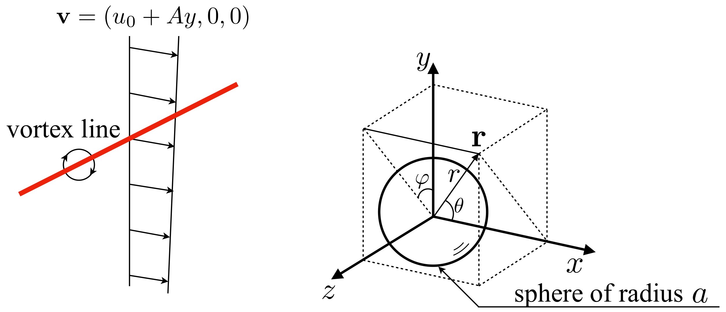
Fig. 9.2 Sphere in weak shear flow.

Let us follow the former analysis by Auton. The pressure distribution at the sphere surface required for calculation the lift can be obtained by Bernoulli’s equation once the velocity distribution is known. The perturbation in the velocity field due to weak shear is assumed to be small, i.e.,

(9.103)\[ \frac{a A}{u_{0}} \ll 1\]

The velocity field is therefore written as the superposition of a primary irrotational flow \(\mathbf{V}\) and a small perturbation \(\mathbf{v}'\) which is proportional to \(a A\):

(9.104)\[ \mathbf{v} = \mathbf{V} + \mathbf{v}'\]

The primary flow is irrotational. Therefore,

(9.105)\[ \nabla \times \mathbf{V} = 0\]

and boundary conditions for \(\mathbf{V}\) are given by

(9.106)\[ \mathbf{n} \cdot \mathbf{V} = 0~~~~\text{at}~r = a\]

(9.107)\[ \mathbf{V} = (u_{0}, 0, 0)~~~\text{as}~r \rightarrow \infty\]

The stream function of the primary flow is given by potential flow theory, i.e.,

(9.108)\[ \psi = \frac{1}{2} r^{2} u_{0} \left( 1 - \frac{a^{3}}{r^{3}} \right) \sin^{2} \theta\]

from which we have

Flows having axial symmetry can be expressed by Stokes’ stream function, for which the velocity components are given by

\(v_{r} = \frac{1}{r^{2} \sin \theta} \frac{\partial \psi}{\partial \theta},~~~~v_{\theta} = - \frac{1}{r \sin \theta} \frac{\partial \psi}{\partial r}\)

(9.109)\[\begin{split} &V_{r} = u_{0} \cos \theta \left( 1 - \frac{a^{3}}{r^{3}} \right) &V_{\theta} = - u_{0} \sin \theta \left( 1 + \frac{a^{3}}{2 r^{3}} \right) &V_{\varphi} = 0 \end{split}\]

\(\psi = \text{const.}\) represents a streamline. It is convenient to absorb the factor \(u_{0}/2\) into the constant, giving

(9.110)\[ r^{2} \left( 1 - \frac{a^{3}}{r^{3}} \right) \sin^{2} \theta = \hat{\rho}_{0}^{2}\]

since \(\hat{\rho}_{0}\) represents the distance between the streamline and the \(x\) axis in the far upstream of the sphere.

Taking \(a/r \rightarrow 0\) yields \(\hat{\rho}_{0} = r \sin \theta\).

Since the flow is steady, the streamline corresponds to the particle path. Therefore, the fluid particle at \(\hat{\rho}_{0}\) in the far upstream moves along this streamline. In this context, the initial coordinate \(\hat{\rho}_{0}\) can be regarded as a label of fluid particle.

By substituting \(\mathbf{v} = \mathbf{V} + \mathbf{v}'\) into the vorticity equation

(9.111)\[ \mathbf{v} \cdot \nabla \boldsymbol{\omega} = \boldsymbol{\omega} \cdot \nabla \mathbf{v}\]

we have

(9.112)\[ ( \mathbf{V} + \mathbf{v}' ) \cdot \nabla \boldsymbol{\omega} = \boldsymbol{\omega} \cdot \nabla ( \mathbf{V} + \mathbf{v}' )\]

By omitting the second order terms, we obtain

By scaling the velocities and vorticity as \(\mathbf{V}^{*} = \mathbf{V} / u_{0}\), \(\mathbf{v}'^{*} = \mathbf{v}' / (aA)\), \(\boldsymbol{\omega}^{*} = \boldsymbol{\omega} / A\) and \(\nabla^{*} = a \nabla\), we have

\(( \mathbf{V} + \mathbf{v}' ) \cdot \nabla \boldsymbol{\omega} = \frac{u_{0}^{2}}{a^{2}} \left\{ \frac{a A}{u_{0}} \mathbf{V}^{*} + \left( \frac{a A}{u_{0}} \right)^{2} \mathbf{v}'^{*} \right\} \cdot \nabla^{*} \boldsymbol{\omega}^{*}\)

(9.113)\[ \mathbf{V} \cdot \nabla \boldsymbol{\omega} = \boldsymbol{\omega} \cdot \nabla \mathbf{V}\]

This equation represents that the vorticity is advected by the primary flow while experiencing stretching also by the primary flow. Lighthill [Lig56a] showed the solution of \(\boldsymbol{\omega}\) expressed in terms of the so-called drift function, \(t\), which is defined by

(9.114)\[ dt = \frac{dx}{V_{x}} = \frac{dy}{V_{y}} = \frac{dz}{V_{z}}\]

with

(9.115)\[ t - \frac{x}{u_{0}} \rightarrow 0~~~~\text{as}~x \rightarrow -\infty\]

Isosurfaces of \(t = \text{const.}\) represent the deformation of material surfaces initially perpendicular to the \(x\) axis in the far upstream. In the spherical polar coordinate system,

(9.116)\[ dt = \frac{dr}{V_{r}} = \frac{rd\theta}{V_{\theta}} \]

Using Eq. (9.109), we have

(9.117)\[ u_{0} dt = - \frac{rd\theta}{\sin \theta \left( 1 + \frac{a^{3}}{2 r^{3}} \right)} \]

By integrating this equation, we can obtain the drift function as \(t(\hat{\rho}_{0}, \theta)\).

The form of Eq. (9.117) may meet singularities at \(\theta = 0\) and \(\pi\), which cause difficulties in numerical integration. Cousins (1970) therefore proposed the following form to avoid the difficulty:

\(u_{0} dt = \left\{ - \frac{\hat{\rho}_{0}}{\sin^{2} \theta} + \left( \frac{\hat{\rho}_{0}}{\sin^{2} \theta} - \frac{r}{\sin \theta \left( 1 + a^{3}/2 r^{3} \right)} \right) \right\} d\theta\)

Integrating this equation from \(\theta = \pi\)~(\(x \rightarrow -\infty\)) to \(0\)~(\(x \rightarrow \infty\)) gives

\(u_{0} t = \frac{\hat{\rho}_{0}}{\tan \theta} - \int_{\theta}^{\pi} \left( \frac{\hat{\rho}_{0}}{\sin^{2} \theta'} - \frac{r'}{\sin \theta' \left( 1 + a^{3}/2 r'^{3} \right)} \right) d\theta'\)

\(1 / \sin \theta'\) diverges at \(\theta = 0\) and \(\pi\), but the sum of the two terms of the integrand approaches zero at these limits, so that the contributions at \(\theta = 0\) and \(\pi\) can be removed when numerical integration is carried out. The parameter \(r'\) also changes during the integration for \(\theta'\). By the streamline equation, Eq. (9.110),

\(r'^{2} \left( 1 - \frac{a^{3}}{r'^{3}} \right) = \frac{\hat{\rho}_{0}^{2}}{\sin^{2} \theta'}\)

\(r'\) can be obtained as the positive root of this equation for given \(\theta'\).

Then, the vorticity is given by (see derivation by Lighthill in Appendix Vorticity in terms of drift function)

(9.118)\[\begin{split}\begin{split} &\omega_{r} = A \sin \varphi \left( V_{r} \left( \frac{\partial t}{\partial \hat{\rho}_{0}} \right)_{\theta} - \left( \frac{\partial r}{\partial \hat{\rho}_{0}} \right)_{\theta} \right) \\ &\omega_{\theta} = A \sin \varphi \left( V_{\theta} \left( \frac{\partial t}{\partial \hat{\rho}_{0}} \right)_{\theta} \right) \\ &\omega_{\varphi} = - A \cos \varphi \frac{r \sin \theta}{\hat{\rho}_{0}} \end{split}\end{split}\]

It is worth noting that \(\omega_{\varphi}\) does not depend on \(t\); the factor \(r \sin \theta / \hat{\rho}_{0} = \hat{\rho} d \varphi / \hat{\rho}_{0} d\varphi\) represents the stretching rate of vorticity (fluid material) element, so the primary flow causes only stretching of the ring vorticity, \(\omega_{\varphi}\). Fig. 9.3 shows a vortex line coming from upstream stretched by the primary flow while advected toward downstream.

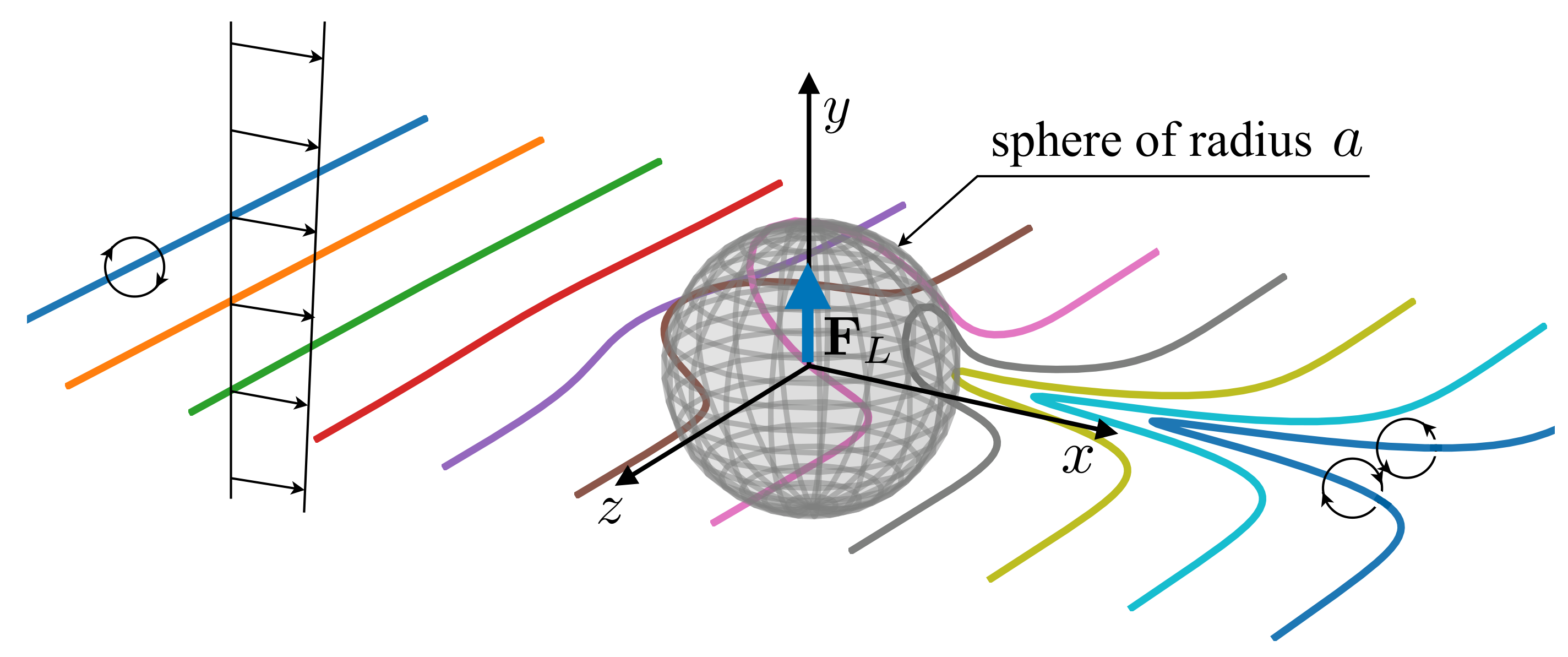
Fig. 9.3 Vortex line stretched by primary flow. \(u_{0} = 1\), \(a = 1\), the initial position of the line element \(y_{0} = 0.1\).

Lighthill [Lig56b] pointed out that the Biot-Savart field should be constructed by the vorticity change

(9.119)\[ \boldsymbol{\omega}_{1} = \boldsymbol{\omega} - \boldsymbol{\omega}_{0}\]

and the Biot-Savart integral does not converge if the uniform oncoming vorticity \(\boldsymbol{\omega}_{0} = (0, 0, -A)\) is not subtracted. The orthogonal matrix

(9.120)\[\begin{split} \mathbf{M}^{-1} = \left( \begin{array}{c} \mathbf{e}_{r} \\ \mathbf{e}_{\theta} \\ \mathbf{e}_{\varphi} \\ \end{array} \right) = \left( \begin{array}{rrr} \sin \theta \cos \varphi &\sin \theta \sin \varphi &\cos \theta \\ \cos \theta \cos \varphi &\cos \theta \sin \varphi &-\sin \theta \\ -\sin \varphi &\cos \varphi &0 \end{array} \right)\end{split}\]

transforms the Cartesian components to the components in the spherical polar coordinate system. With this matrix,

(9.121)\[\begin{split} \boldsymbol{\omega}_{0} \rightarrow \left( \begin{array}{c} \omega_{0r} \\ \omega_{0\theta} \\ \omega_{0\varphi} \end{array} \right) = \mathbf{M}^{-1} \left( \begin{array}{c} \omega_{0y} \\ \omega_{0z} \\ \omega_{0x} \end{array} \right) = \mathbf{M}^{-1} \left( \begin{array}{r} 0 \\ -A \\ 0 \end{array} \right) = \left( \begin{array}{c} -A \sin \varphi \sin \theta \\ -A \sin \varphi \cos \theta \\ -A \cos \varphi \end{array} \right)\end{split}\]

Thus,

(9.122)\[\begin{split}\begin{split} &\omega_{1r} = A \sin \varphi \left\{ \left( V_{r} \left( \frac{\partial t}{\partial \hat{\rho}_{0}} \right)_{\theta} - \left( \frac{\partial r}{\partial \hat{\rho}_{0}} \right)_{\theta} \right) + \sin \theta \right\} \\ &\omega_{1\theta} = A \sin \varphi \left\{ \left( V_{\theta} \left( \frac{\partial t}{\partial \hat{\rho}_{0}} \right)_{\theta} \right) + \cos \theta \right\} \\ &\omega_{1\varphi} = A \cos \varphi \left\{ - \frac{r \sin \theta}{\hat{\rho}_{0}} + 1 \right\} \end{split}\end{split}\]

The secondary velocity field \(\mathbf{v}'\) can then be constructed from four parts: \begin{itemize} \item the uniform shear flow perturbation \(\mathbf{v}_{0}^{e} = (Ay, 0, 0)\), \item an irrotational flow field, \(\mathbf{v}_{0}^{i}\), enforcing \(\mathbf{v}_{0}~(=\mathbf{v}_{0}^{e} + \mathbf{v}_{0}^{i})\) so as to satisfy the boundary condition \(\mathbf{n} \cdot \mathbf{v}_{0} = \mathbf{n} \cdot ( \mathbf{v}_{0}^{e} + \mathbf{v}_{0}^{i} ) = 0\) at \(r = a\), \item the Biot-Savart field, \(\mathbf{v}_{1}^{e}\), by \(\boldsymbol{\omega}_{1}\), \item an irrotational flow field, \(\mathbf{v}_{1}^{i}\), enforcing \(\mathbf{v}_{1}~(=\mathbf{v}_{1}^{e} + \mathbf{v}_{1}^{i})\) so as to satisfy the boundary condition \(\mathbf{n} \cdot \mathbf{v}_{1} = \mathbf{n} \cdot ( \mathbf{v}_{1}^{e} + \mathbf{v}_{1}^{i} ) = 0\) at \(r = a\). \end{itemize} The first one in the spherical polar coordinate system is written as

(9.123)\[\begin{split} \mathbf{v}_{0}^{e} \rightarrow \left( \begin{array}{c} v_{0r}^{e} \\ v_{0\theta}^{e} \\ v_{0\varphi}^{e} \end{array} \right) = \mathbf{M}^{-1} \left( \begin{array}{c} v_{0y} \\ v_{0z} \\ v_{0x} \end{array} \right) = \mathbf{M}^{-1} \left( \begin{array}{c} 0 \\ 0 \\ A r \sin \theta \cos \varphi \end{array} \right) = \left( \begin{array}{c} A r \sin \theta \cos \theta \cos \varphi \\ -A r \sin^{2} \theta \cos \varphi \\ 0 \end{array} \right)\end{split}\]

\(\mathbf{v}_{0}^{i}\) is deduced from the following velocity potential:

(9.124)\[ \phi_{0}^{i} = \frac{A a^{5}}{3 r^{3}} \sin \theta \cos \theta \cos \varphi\]

from which

(9.125)\[ \mathbf{v}_{0}^{i} = \nabla \phi_{0}^{i} = \frac{\partial \phi}{\partial r} \mathbf{e}_{r} + \frac{1}{r} \frac{\partial \phi}{\partial \theta} \mathbf{e}_{\theta} + \frac{1}{r \sin \theta} \frac{\partial \phi}{\partial \varphi} \mathbf{e}_{\varphi}\]

and

(9.126)\[\begin{split}\begin{split} &v_{0r}^{i} = - \frac{A a^{5}}{r^{4}} \sin \theta \cos \theta \cos \varphi \\ &v_{0\theta}^{i} = \frac{A a^{5}}{3 r^{4}} \cos \varphi \cos 2 \theta \\ &v_{0\varphi}^{i} = - \frac{A a^{5}}{3 r^{4}} \cos \theta \sin \varphi \end{split}\end{split}\]

Hence,

(9.127)\[\begin{split}\begin{split} &v_{0r} = A r \sin \theta \cos \theta \cos \varphi \left( 1 - \frac{a^{5}}{r^{5}} \right) \\ &v_{0\theta} = A r \cos \varphi \left( -\sin^{2} \theta + \frac{a^{5}}{3 r^{5}} \cos 2 \theta \right) \\ &v_{0\varphi} = - \frac{A a^{5}}{3 r^{4}} \cos \theta \sin \varphi \end{split}\end{split}\]

It is obvious that \(v_{0r} = 0\) at \(r = a\).

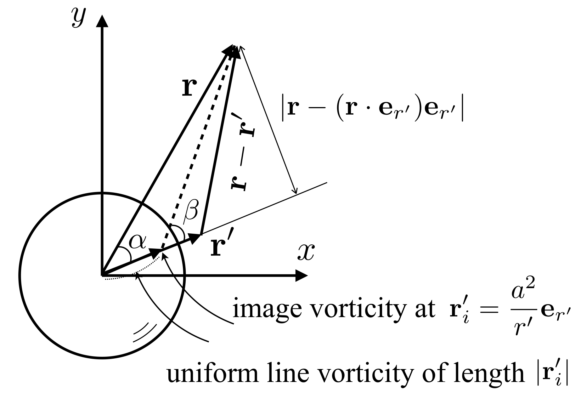
Fig. 9.4 Image system of vorticity

The Biot-Savart field \(\mathbf{v}_{1}^{e}\) induced by \(\boldsymbol{\omega}_{1}\) is given as

(9.128)\[ \mathbf{v}_{1}^{e} (\mathbf{r}) = \frac{1}{4 \pi} \iiint_{V'} \frac{\boldsymbol{\omega}_{1}(\mathbf{r}') \times (\mathbf{r} - \mathbf{r}')}{|\mathbf{r} - \mathbf{r}'|^{3}} dV'\]

Lighthill [Lig56b] showed that \(\mathbf{v}_{1}^{i}\) is given as the Biot-Savart field of a system of image vorticity inside the sphere, that is, for \(\boldsymbol{\omega_{1}} dV\) at \((r, \theta, \varphi)\) external to the sphere, an image system of vorticity at the image point \((a^{2}/r, \theta, \varphi)\)

(9.129)\[ \boldsymbol{\omega}_{i} dV = \left( \frac{a}{r} \omega_{1r}, - \frac{a}{r} \omega_{1\theta}, - \frac{a}{r} \omega_{1\varphi} \right) dV\]

and a uniform line vortex of strength

(9.130)\[ \boldsymbol{\omega}_{l} dV = \left( - \frac{1}{a} \omega_{1r}, 0, 0 \right) dV\]

between the center of the sphere and the position of the image vorticity (see Fig. 9.4). The position, \(\mathbf{r}'_{i}\), of the image system for \(\mathbf{r}'\) can be written in the vectorial form as

\[\begin{equation*} \mathbf{r}'_{i} = \frac{a^{2}}{r'} \mathbf{e}_{r'} \end{equation*}\]

where

(9.131)\[ \mathbf{e}_{r'} = \frac{\mathbf{r}'}{r'}\]

At \(\mathbf{r}'_{i}\), the image vorticity can be written as

(9.132)\[ \boldsymbol{\omega}_{i} = - \frac{a}{r'} \left\{ \boldsymbol{\omega}_{1}(\mathbf{r}') - 2 ( \boldsymbol{\omega}_{1}(\mathbf{r}') \cdot \mathbf{e}_{r'} ) \mathbf{e}_{r'} \right\}\]

Therefore, the contribution of \(\boldsymbol{\omega}_{i}\) to the Biot-Savart integral is expressed by (Appendix Biot-Savart field by uniform line vorticity)

(9.133)\[ \frac{1}{4 \pi} \iiint_{V'} \frac{\boldsymbol{\omega}_{i} \times (\mathbf{r} - \mathbf{r}'_{i})}{|\mathbf{r} - \mathbf{r}'_{i}|^{3}} dV' \]

Then the uniform line vortex is expressed as

(9.134)\[ \boldsymbol{\omega}_{l} = - \frac{\boldsymbol{\omega}_{1}(\mathbf{r}') \cdot \mathbf{e}_{r'}}{a}\]

It should be noted that the line vorticity is the strength of vorticity per unit length. Being similar to the Biot-Savart integral for a line current, we can write the Biot-Savart integral for the uniform line vortex as (see Biot-Savart field by uniform line vorticity)

(9.135)\[ \frac{1}{4 \pi} \iiint_{V'} \frac{\boldsymbol{\omega}_{l} \times \mathbf{r}}{|\mathbf{r} - (\mathbf{r} \cdot \mathbf{e}_{r'}) \mathbf{e}_{r'}|^{2}} \left( \mathbf{e}_{r} \cdot \mathbf{e}_{r'} - \frac{(\mathbf{r} - \mathbf{r}'_{i}) \cdot \mathbf{r}'}{|(\mathbf{r} - \mathbf{r}'_{i}) \cdot \mathbf{r}'|} \right) dV' \]

Thus,

(9.136)\[ \mathbf{v}_{1}^{i} (\mathbf{r}) = \frac{1}{4 \pi} \iiint_{V'} \left\{ \frac{\boldsymbol{\omega}_{i} \times (\mathbf{r} - \mathbf{r}'_{i})}{|\mathbf{r} - \mathbf{r}'_{i}|^{3}} + \frac{\boldsymbol{\omega}_{l} \times \mathbf{r}}{|\mathbf{r} - (\mathbf{r} \cdot \mathbf{e}_{r'}) \mathbf{e}_{r'}|^{2}} \left( \mathbf{e}_{r} \cdot \mathbf{e}_{r'} - \frac{(\mathbf{r} - \mathbf{r}'_{i}) \cdot \mathbf{r}'}{|(\mathbf{r} - \mathbf{r}'_{i}) \cdot \mathbf{r}'|} \right) \right\} dV'\]

and

(9.137)\[ \mathbf{v}_{1} (\mathbf{r}) = \frac{1}{4 \pi} \iiint_{V'} \left\{ \frac{\boldsymbol{\omega}_{1}(\mathbf{r}') \times (\mathbf{r} - \mathbf{r}')}{|\mathbf{r} - \mathbf{r}'|^{3}} + \frac{\boldsymbol{\omega}_{i} \times (\mathbf{r} - \mathbf{r}'_{i})}{|\mathbf{r} - \mathbf{r}'_{i}|^{3}} + \frac{\boldsymbol{\omega}_{l} \times \mathbf{r}}{|\mathbf{r} - (\mathbf{r} \cdot \mathbf{e}_{r'}) \mathbf{e}_{r'}|^{2}} \left( \mathbf{e}_{r} \cdot \mathbf{e}_{r'} - \frac{(\mathbf{r} - \mathbf{r}'_{i}) \cdot \mathbf{r}'}{|(\mathbf{r} - \mathbf{r}'_{i}) \cdot \mathbf{r}'|} \right) \right\} dV'\]

Auton obtained the Biot-Savart field by means of numerical integration, in which some elaborative variable transformation were used to avoid singularities and sharp behaviors of the integrand. Once \(\mathbf{v}_{1}\) is obtained, the secondary velocity field can be obtained as

(9.138)\[ \mathbf{v}' = \mathbf{v}_{0} + \mathbf{v}_{1}\]

Fig. 9.5 shows the velocity components of the secondary flow given by Auton.

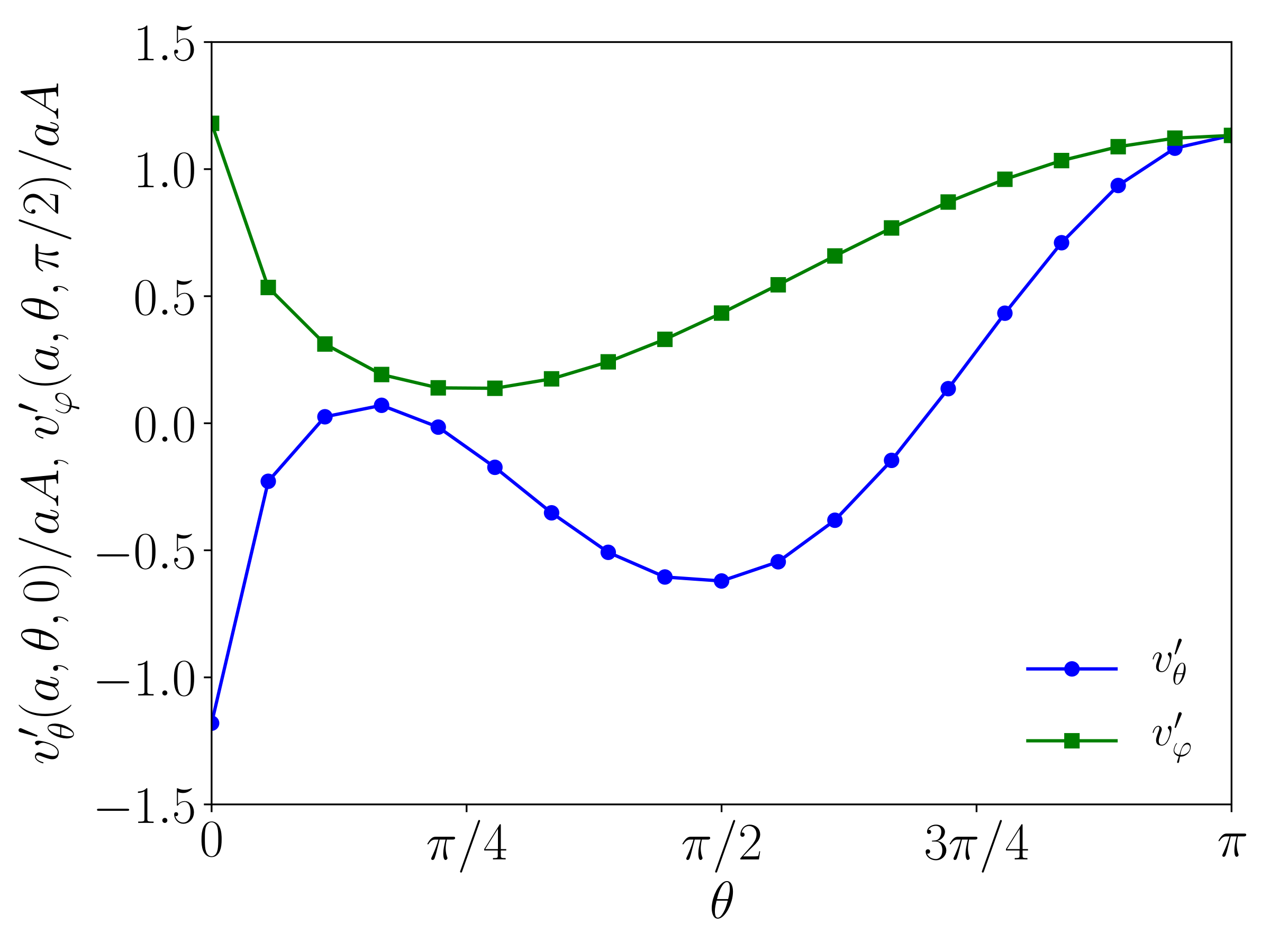
Fig. 9.5 Secondary velocity at sphere surface produced by vorticity, \(v'_{\theta}(a, \theta, 0)\) and \(v'_{\varphi}(a, \theta, \pi/2)\).

The lift force acting on the sphere is calculated by

(9.139)\[ \mathbf{F} = \iint_{S} - p \mathbf{n} dS\]

Bernoulli’s theorem shows that

(9.140)\[ p = p_{0} + \frac{1}{2} \rho u_{0}^{2} - \frac{1}{2} \rho \mathbf{v} \cdot \mathbf{v}\]

where \(p_{0}\) is the pressure in the far upstream on the stagnation streamline. For the velocity square,

(9.141)\[ \mathbf{v} \cdot \mathbf{v} = ( \mathbf{V} + \mathbf{v}' ) \cdot ( \mathbf{V} + \mathbf{v}' ) = ( V_{r} + v'_{r} )^{2} + ( V_{\theta} + v'_{\theta} )^{2} + ( V_{\varphi} + v'_{\varphi} )^{2}\]

Since \(V_{r} = v_{r} = 0\) at \(r = a\) and \(V_{\varphi} = 0\) due to symmetry this reduces to

(9.142)\[ \mathbf{v} \cdot \mathbf{v} = V_{\theta}^{2} + 2 V_{\theta} v'_{\theta} + O((aA)^{2})\]

Therefore, to the first order,

(9.143)\[ p = p_{0} + \frac{1}{2} \rho u_{0}^{2} - \frac{1}{2} \rho V_{\theta}^{2} - \rho V_{\theta} v'_{\theta} \]

However, the first two terms are constant and have no contributions to the integral.

Indenticaly, \(\iint_{S} (~\text{const.}~) \mathbf{n} dS = 0\) for the closed surfaces.

In addition, the potential component, \(V_{\theta}\), is symmetric, and therefore, the integral vanishes for this. Hence, only the fourth term in the pressure survives after integration.

(9.144)\[ \mathbf{F} = \iint_{S} \rho V_{\theta} v'_{\theta} \mathbf{n} dS\]

From Eq. (9.109),

(9.145)\[ V_{\theta} = - \frac{3}{2} u_{0} \sin \theta~~~~\text{at}~r = a\]

According to the dependence of Eq. (9.122) on \(\varphi\), we can write

(9.146)\[ \boldsymbol{\omega}_{1}(\hat{\rho}'_{0}, \theta', \varphi') = \boldsymbol{\omega}_{1}(\hat{\rho}'_{0}, \theta', 0) \cos \varphi' +\boldsymbol{\omega}_{1}(\hat{\rho}'_{0}, \theta', \pi/2) \sin \varphi'\]

This dependence on \(\varphi\) results in a similar form of the perturbed velocity field:

(9.147)\[ \mathbf{v}_{1}(r, \theta, \varphi) = \mathbf{v}_{1}(r, \theta, 0) \cos \varphi + \mathbf{v}_{1}(r, \theta, \pi/2) \sin \varphi\]

In particular, for the \(\theta\) component,

(9.148)\[ v'_{\theta}(a, \theta, \varphi) = v'_{\theta}(a, \theta, 0) \cos \varphi\]

The \(y\) component of the lift is therefore given by

(9.149)\[ F_{y} = \iint_{S} \rho V_{\theta} v'_{\theta} \mathbf{n} dS = - \rho \frac{3}{2} u_{0} a^{2} \int_{0}^{2\pi} \int_{0}^{\pi} v'_{\theta}(a, \theta, 0) \sin^{2} \theta \cos \varphi \mathbf{n} d \theta d\varphi\]

The Cartesian components of the unit normal are

(9.150)\[\begin{split} \mathbf{n} = \left( \begin{array}{c} n_{x}\\ n_{y}\\ n_{z} \end{array} \right) = \left( \begin{array}{c} \cos \theta\\ \sin \theta \cos \varphi\\ \sin \theta \sin \varphi \end{array} \right)\end{split}\]

Substituting this expression into the lift equation yields

For the integration for \(\varphi\), \(\int_{0}^{2\pi} \cos^{2} \varphi d\varphi = \pi\). A numerical integration for the \(\theta\) term gives \(\int_{0}^{\theta} v'_{\theta} (a, \theta, 0) \sin^{2} \theta d\theta \sim -0.44456\)

(9.151)\[ F_{y} = - \frac{3}{2} \rho u_{0} a^{2} \int_{0}^{2\pi} \cos^{2} \varphi d\varphi \int_{0}^{\pi} v'_{\theta}(a, \theta, 0) \sin^{3} \theta d\theta = - \frac{3}{2} \rho u_{0} \pi a^{2} \int_{0}^{\pi} v'_{\theta}(a, \theta, 0) \sin^{3} \theta d\theta\]

Auton prepared a lookup table of \(v'_{\theta}(a, \theta, 0) / a A\) for integrating \(F_{y}\) and obtained

(9.152)\[ F_{y} \sim 2.09454 \rho a^{3} u_{0} A = 0.500035 \cdot \rho \frac{4 \pi a^{3}}{3} u_{0} A\]

The value of the lift coefficient was confirmed to be exactly \(1/2\) by means of the momentum-integral theory.

Legendre and Magnaudet [LM97] derived the following lift coefficient of sphere in the Stokes regime:

(9.153)\[C_{L} = \frac{6}{\pi^{2}} \frac{2.255}{\sqrt{Sr Re} \left[ 1 + 0.2 Re/Sr \right]^{3/2}}\]

where \(Sr~(= 2 a A / u_{0})\) is the dimensionless shear rate of the incident flow. Then, they carried out numerical simulation of a weak shear flow past a spherical bubble at various Reynolds numbers and showed that the lift coefficient approaches Auton’s result at high Reynolds numbers Legendre and Magnaudet [LM98]. The numerical results were used to connect Eq. (10.40) and the Auton lift, that is,

(9.154)\[C_{L} = \left( \left[ \frac{6}{\pi^{2}} \frac{2.255}{\sqrt{Sr Re} \left[ 1 + 0.2 Re/Sr \right]^{3/2}} \right]^{2} + \left[ \frac{1}{2} \left( \frac{1 + 16/Re}{1 + 29/Re} \right) \right]^{2} \right)^{1/2}\]