Continuity and NS equations in polar coordinate systems

Referred from

Drag acting on a solid sphere in Stokes flow (GKB)

Differentiation of vectors

Orthogonal curvilinear coordinates

Polar coordinates, e.g., the cylindrical and spherical coordinates, are useful when dealing with flow fields symmetric with respect to an axis or a point. We need expressions of the differential operators such as \(grad\), \(div\) and \(rot\) to establish the continuity and Navier-Stokes equations in polar coordinate systems.

The cylindrical coordinate \((r, \theta, z)\) system, where the coordinates are written in the order to construct the right-handed system, is given by

(63)\[\begin{split}\begin{split} &x = r \cos \theta \\ &y = r \sin \theta \\ &z = z \end{split}\end{split}\]

The spherical coordinates \((r, \theta, \phi)\) system is given by

(64)\[\begin{split}\begin{split} &x = r \sin \theta \cos \phi \\ &y = r \sin \theta \sin \phi \\ &z = r \cos \theta \\ \end{split}\end{split}\]

The base vectors in these coordinate systems are obtained by differentiating the position vector \(\mathbf{r}\) along the coordinate lines. Therefore in the cylindrical coordinates

(65)\[\begin{split}\begin{split} &\mathbf{e}_{r} = \frac{\partial \mathbf{r}}{\partial r} = \cos \theta \mathbf{e}_{x} + \sin \theta \mathbf{e}_{y} = (\cos \theta, \sin \theta, 0) \\ &\mathbf{e}_{\theta} = \frac{1}{r} \frac{\partial \mathbf{r}}{\partial \theta} = - \sin \theta \mathbf{e}_{x} + \cos \theta \mathbf{e}_{y} = (-\sin \theta, \cos \theta, 0) \\ &\mathbf{e}_{z} = \frac{\partial \mathbf{r}}{\partial z} = \mathbf{e}_{z} = (0, 0, 1) \end{split}\end{split}\]

and in the spherical coordinates

(66)\[\begin{split}\begin{split} &\mathbf{e}_{r} =\frac{\partial \mathbf{r}}{\partial r}=\sin \theta \cos \varphi \mathbf{e}_{x}+\sin \theta \sin \varphi \mathbf{e}_{y}+\cos \theta \mathbf{e}_{z} = ( \sin \theta \cos \varphi, \sin \theta \sin \varphi, \cos \theta ) \\ &\mathbf{e}_{\theta}=\frac{1}{r} \frac{\partial \mathbf{r}}{\partial \theta}=\cos \theta \cos \varphi \mathbf{e}_{x} + \cos \theta \sin \varphi \mathbf{e}_{y} - \sin \theta \mathbf{e}_{z} = (\cos \theta \cos \varphi, \cos \theta \sin \varphi, - \sin \theta) \\ &\mathbf{e}_{\varphi} =\frac{1}{r \sin \theta} \frac{\partial \mathbf{r}}{\partial \varphi}=- \sin \varphi \mathbf{e}_{x} + \cos \varphi \mathbf{e}_{y} = (- \sin \varphi, \cos \varphi, 0) \end{split}\end{split}\]

It can be immediately confirmed that the base vectors are orthogonal each other by taking the dot products of them. The coordinate lines are curved, while the coordinate lines are orthogonal. Such coordinate systems are called orthogonal curvilinear coordinate systems.

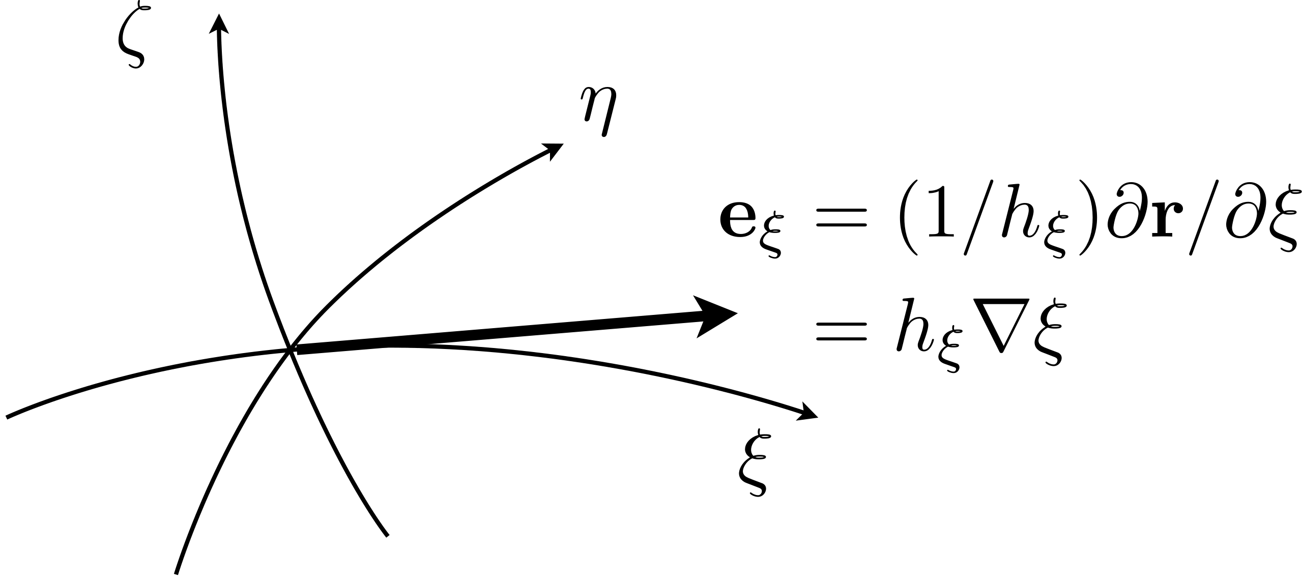
We will derive the differential operators for these polar coordinate system. However, let us begin by a general manner. Let \(\xi, \eta, \zeta\) are orthogonal curvilinear coordinates constructing the right-handed system as shown in Fig. 4. For instance, \(r \rightarrow \xi\), \(\theta \rightarrow \eta\), \(\phi \rightarrow \zeta\) for the spherical coordinate system. The Cartesian coordinate systems can be expressed in terms of the curvilinear coordinates:

(67)\[\begin{split}\begin{split} &x = f(\xi, \eta, \zeta) \\ &y = g(\xi, \eta, \zeta) \\ &z = h(\xi, \eta, \zeta) \end{split}\end{split}\]

Solving these for \(\xi, \eta, \zeta\) yields

(68)\[\begin{split}\begin{split} &\xi = F(x,y,z) \\ &\eta = G(x,y,z) \\ &\zeta = H(x,y,z) \end{split}\end{split}\]

The inverse transformation with one-to-one correspondence is possible when the following Jacobian is not zero:

(69)\[\begin{split}J = \left| \begin{array}{ccc} \frac{\partial x}{\partial \xi} &\frac{\partial x}{\partial \eta} &\frac{\partial x}{\partial \zeta} \\ \frac{\partial y}{\partial \xi} &\frac{\partial y}{\partial \eta} &\frac{\partial y}{\partial \zeta} \\ \frac{\partial z}{\partial \xi} &\frac{\partial z}{\partial \eta} &\frac{\partial z}{\partial \zeta} \\ \end{array} \right|\end{split}\]

The Jacobian is the coefficient of a infinitesimal volume in the curvilinear coordinate system:

(70)\[dV = J d\xi d\eta d\zeta\]

Fig. 4 Orthogonal curvilinear system

Length of line element and base vectors

In the Cartesian coordinate system, the square, \(ds^{2}\), of a line element is given by

(71)\[ds^{2} = d \mathbf{r} \cdot d \mathbf{r} = dx_{i} dx_{i} = dx^{2} + dy^{2} + dz^{2}\]

The length, of course, can also be measured by making use of the curvilinear coordinates, and the value should be the same in both coordinate system. The invariance of \(ds^{2}\) is therefore the starting point of the theory. Due to the functional relationships of the coordinate transformation,

(72)\[dx_{i} = \frac{\partial x_{i}}{\partial \xi_{j}} d \xi_{j}\]

Hence, \(ds^{2}\) can be written as

(73)\[ds^{2} = dx_{i} dx_{i} = \frac{\partial x_{i}}{\partial \xi_{j}} \frac{\partial x_{i}}{\partial \xi_{k}} d \xi_{j} d \xi_{k}\]

The coefficient, \(d\xi_{j} d\xi_{k}\), in the right-most equation

(74)\[\frac{\partial x_{i}}{\partial \xi_{j}} \frac{\partial x_{i}}{\partial \xi_{k}} = \frac{\partial \mathbf{r}}{\partial \xi_{j}} \cdot \frac{\partial \mathbf{r}}{\partial \xi_{k}}\]

is the dot product between vectors tangent to the coordinate lines \(\xi_{j}\) and \(\xi_{k}\).

the magnitudes of the vectors are not unity.

However, the dot product gives zero if \(j \neq k\) due to the orthogonality of the coordinate lines. Therefore,

(75)\[ds^{2} = ( h_{\xi} d\xi )^{2}+ ( h_{\eta} d\eta )^{2}+ ( h_{\zeta} d\zeta )^{2}\]

where

(76)\[h_{i}^{2} = \frac{\partial \mathbf{r}}{\partial \xi_{i}} \cdot \frac{\partial \mathbf{r}}{\partial \xi_{i}}~~~~\text{no sum on }i\]

The cylindrical coordinate system uses the azimuthal angle \(\theta\) for \(\eta\). The differential, \(d\theta\), does not have the dimension of the length, but \(r d\theta\) does. The coefficients, \(h_{\xi}, h_{\eta}, h_{\zeta}\), convert the differentials of the curvilinear coordinates so as to have the length dimensions; they are called metric.

Let us make the base vectors, \(\mathbf{e}_{\xi}, \mathbf{e}_{\eta}, \mathbf{e}_{\zeta}\), which are the derivatives of \(\mathbf{r}\) along the coordinates. The base vector \(\mathbf{e}_{\xi}\) is obtained by differentiating \(\mathbf{r}\) with respect to \(\xi\). However, as shown in the equation of \(ds^{2}\), the length of a line element along \(\xi\) is \(h_{\xi} d\xi\). Therefore,

(77)\[\mathbf{e}_{\xi} = \frac{1}{h_{\xi}} \frac{\partial \mathbf{r}}{\partial \xi},~~ \mathbf{e}_{\eta} = \frac{1}{h_{\eta}} \frac{\partial \mathbf{r}}{\partial \eta},~~ \mathbf{e}_{\zeta} = \frac{1}{h_{\zeta}} \frac{\partial \mathbf{r}}{\partial \zeta}\]

On the other hand, \(\nabla \xi\) is a vector field normal to iso-surfaces of \(\xi = \text{const.}\) in other words \(\eta \zeta\) surfaces. The coordinate line \(\xi\) is also orthogonal to the \(\eta \zeta\) surface. Therefore, \(\nabla \xi\) is also tangent to the \(\xi\) line and parallel to \(\mathbf{e}_{\xi}\). Let \(C\) is the ratio of the magnitudes of \(\mathbf{e}_{\xi}\) and \(\nabla \xi\). Hence,

(78)\[\nabla \xi = C \mathbf{e}_{\xi} = C \frac{1}{h_{\xi}} \frac{\partial \mathbf{r}}{\partial \xi}\]

Taking inner product with \(\frac{1}{h_{\xi}} \frac{\partial \mathbf{r}}{\partial \xi}\) yields

(79)\[\frac{\partial \mathbf{r}}{\partial \xi} \cdot \nabla \xi = C \frac{1}{h_{\xi}} \frac{\partial \mathbf{r}}{\partial \xi} \cdot \frac{\partial \mathbf{r}}{\partial \xi} = C h_{\xi}\]

Since the first equation is \(1\), \(C = 1/h_{\xi}\). Hence,

(80)\[\nabla \xi = \frac{\mathbf{e}_{\xi}}{h_{\xi}},~~ \nabla \eta = \frac{\mathbf{e}_{\eta}}{h_{\eta}},~~ \nabla \zeta = \frac{\mathbf{e}_{\zeta}}{h_{\zeta}}\]

The base vectors in the \(\xi\eta\zeta\) coordinate system have become clear. Let us write a vector field \(\mathbf{f}\) in the orthogonal coordinate system as

(81)\[\mathbf{f} = f_{\xi} \mathbf{e}_{\xi} + f_{\eta} \mathbf{e}_{\eta} + f_{\zeta} \mathbf{e}_{\zeta}\]

\(f_{\xi}, f_{\eta}, f_{\zeta}\) are the components of \(\mathbf{f}\) in the \(\xi, \eta, \zeta\) directions.

Gradient

We are now ready to formulate the differential operators in the orthogonal curvilinear systems. Let us begin by the gradient of scalar field \(\phi\) in the \(\xi\eta\zeta\) coordinate system. The scalar field \(\phi (x,y,z)\) can be written as \(\phi (\xi,\eta,\zeta)\) by coordinate transformation.

The scalar field does not change the value of its component under any coordinate transformation.

Therefore, by the chain rule,

(82)\[\nabla \phi = \frac{\partial \phi}{\partial \xi} \frac{\partial \xi}{\partial \mathbf{r}} +\frac{\partial \phi}{\partial \eta} \frac{\partial \eta}{\partial \mathbf{r}} +\frac{\partial \phi}{\partial \zeta} \frac{\partial \zeta}{\partial \mathbf{r}}\]

Replacing \(\nabla \xi_{i}\) with the base vectors yields the following equation for the gradient:

(83)\[\nabla \phi = \frac{1}{h_{\xi}} \frac{\partial \phi}{\partial \xi} \mathbf{e}_{\xi} +\frac{1}{h_{\eta}} \frac{\partial \phi}{\partial \eta} \mathbf{e}_{\eta} +\frac{1}{h_{\zeta}} \frac{\partial \phi}{\partial \zeta} \mathbf{e}_{\zeta}\]

Divergence and Laplacian

Taking divergence of vector field \(\mathbf{f}\) yields

(84)\[\nabla \cdot \mathbf{f} = \nabla \cdot (f_{\xi} \mathbf{e}_{\xi} + f_{\eta} \mathbf{e}_{\eta} + f_{\zeta} \mathbf{e}_{\zeta})\]

Expanding the first term gives

(85)\[\begin{split}\begin{split} \nabla \cdot (f_{\xi} \mathbf{e}_{\xi} ) &= \nabla \cdot [ f_{\xi} h_{\eta} h_{\zeta} ( \mathbf{e}_{\eta} \times \mathbf{e}_{\zeta} ) ] = \nabla (h_{\eta} h_{\zeta} f_{\xi}) \cdot ( \mathbf{e}_{\eta} \times \mathbf{e}_{\zeta} ) + (h_{\eta} h_{\zeta} f_{\xi}) \nabla \cdot ( \mathbf{e}_{\eta} \times \mathbf{e}_{\zeta} ) \\ &= \nabla (h_{\eta} h_{\zeta} f_{\xi}) \cdot ( \mathbf{e}_{\eta} \times \mathbf{e}_{\zeta} ) \end{split}\end{split}\]

where \(\mathbf{e}_{\xi} = \mathbf{e}_{\eta} \times \mathbf{e}_{\zeta}\) and the identity \(\nabla \cdot (\nabla \phi \times \nabla \psi) = 0\) were used.

(86)\[\begin{split}\begin{split} \nabla (h_{\eta} h_{\zeta} f_{\xi}) \cdot ( \mathbf{e}_{\eta} \times \mathbf{e}_{\zeta} ) &= \frac{1}{h_{\xi}} \frac{\partial (h_{\eta} h_{\zeta} f_{\xi})}{\partial \xi} \mathbf{e}_{\xi} \cdot ( \nabla \eta \times \nabla \zeta ) = \frac{1}{h_{\xi}} \frac{\partial (h_{\eta} h_{\zeta} f_{\xi})}{\partial \xi} \mathbf{e}_{\xi} \cdot ( \frac{\mathbf{e}_{\eta}}{h_{\eta}} \times \frac{\mathbf{e}_{\zeta}}{h_{\zeta}} ) \\ & = \frac{1}{h_{\xi} h_{\eta} h_{\zeta}} \frac{\partial (h_{\eta} h_{\zeta} f_{\xi})}{\partial \xi} \end{split}\end{split}\]

The other terms can also be rewritten in similar forms. Thus, the divergence of \(\mathbf{f}\) is given by

(87)\[\nabla \cdot \mathbf{f} = \frac{1}{h_{\xi} h_{\eta} h_{\zeta}} \left[ \frac{\partial (h_{\eta} h_{\zeta} f_{\xi})}{\partial \xi} +\frac{\partial (h_{\zeta} h_{\xi} f_{\eta})}{\partial \eta} +\frac{\partial (h_{\xi} h_{\eta} f_{\zeta})}{\partial \zeta} \right]\]

The Laplacian of \(\phi\) is obtained by setting \(\mathbf{f} = \nabla \phi\) in the divergence equation:

(88)\[\nabla^{2} \phi = \frac{1}{h_{\xi} h_{\eta} h_{\zeta}} \left[ \frac{\partial }{\partial \xi} \left( \frac{h_{\eta} h_{\zeta}}{h_{\xi}} \right) \frac{\partial \phi}{\partial \xi} +\frac{\partial }{\partial \eta} \left( \frac{h_{\zeta} h_{\xi}}{h_{\eta}} \right) \frac{\partial \phi}{\partial \eta} +\frac{\partial }{\partial \zeta} \left( \frac{h_{\xi} h_{\eta}}{h_{\zeta}} \right) \frac{\partial \phi}{\partial \zeta} \right]\]

Rotation

Taking rotation of \(\mathbf{f}\) yields

(89)\[\nabla \times \mathbf{f} = \nabla \times (f_{\xi} \mathbf{e}_{\xi} + f_{\eta} \mathbf{e}_{\eta} + f_{\zeta} \mathbf{e}_{\zeta})\]

the first term is as follows:

(90)\[\begin{split}\begin{split} \nabla \times (f_{\xi} \mathbf{e}_{\xi} ) &= \nabla \times ( f_{\xi} h_{\xi} \nabla \xi ) = \nabla ( f_{\xi} h_{\xi} ) \times \nabla \xi + f_{\xi} h_{\xi} \nabla \times \nabla \xi = \nabla ( f_{\xi} h_{\xi} ) \times \nabla \xi \\ &= \left( \frac{1}{h_{\xi}} \frac{\partial f_{\xi} h_{\xi}}{\partial \xi} \mathbf{e}_{\xi} +\frac{1}{h_{\eta}} \frac{\partial f_{\xi} h_{\xi}}{\partial \eta} \mathbf{e}_{\eta} +\frac{1}{h_{\zeta}} \frac{\partial f_{\xi} h_{\xi}}{\partial \zeta} \mathbf{e}_{\zeta} \right) \times \nabla \xi \\ &= \left( \frac{1}{h_{\xi}} \frac{\partial f_{\xi} h_{\xi}}{\partial \xi} \mathbf{e}_{\xi} +\frac{1}{h_{\eta}} \frac{\partial f_{\xi} h_{\xi}}{\partial \eta} \mathbf{e}_{\eta} +\frac{1}{h_{\zeta}} \frac{\partial f_{\xi} h_{\xi}}{\partial \zeta} \mathbf{e}_{\zeta} \right) \times \frac{\mathbf{e}_{\xi}}{h_{\xi}} \\ &= -\frac{1}{h_{\xi} h_{\eta}} \frac{\partial f_{\xi} h_{\xi}}{\partial \eta} \mathbf{e}_{\zeta} +\frac{1}{h_{\xi} h_{\zeta}} \frac{\partial f_{\xi} h_{\xi}}{\partial \zeta} \mathbf{e}_{\eta} \end{split}\end{split}\]

The remaining two terms can also be transformed in the same manner. Then, we obtain

(91)\[\begin{split}\begin{split} \nabla \times \mathbf{f} = &\frac{1}{h_{\eta} h_{\zeta}} \left( \frac{\partial h_{\zeta} f_{\zeta}}{\partial \eta} -\frac{\partial h_{\eta} f_{\eta}}{\partial \zeta} \right) \mathbf{e}_{\xi} \\ &+ \frac{1}{h_{\zeta} h_{\xi}} \left( \frac{\partial h_{\xi} f_{\xi}}{\partial \zeta} -\frac{\partial h_{\zeta} f_{\zeta}}{\partial \xi} \right) \mathbf{e}_{\eta} + \frac{1}{h_{\xi} h_{\eta}} \left( \frac{\partial h_{\eta} f_{\eta}}{\partial \xi} -\frac{\partial h_{\xi} f_{\xi}}{\partial \eta} \right) \mathbf{e}_{\zeta} \end{split}\end{split}\]

For exercises, (1) calculate the Jacobian and the metric of the cylindrical and spherical coordinate systems, and (2) confirm that \(J = h_{\xi} h_{\eta} h_{\zeta}\).

The differential operators in the cylindrical coordinate system are

(92)\[\nabla \phi = \frac{\partial \phi}{\partial r} \mathbf{e}_{r} +\frac{1}{r}\frac{\partial \phi}{\partial \theta} \mathbf{e}_{\theta} +\frac{\partial \phi}{\partial z} \mathbf{e}_{z}\]

(93)\[\nabla \cdot \mathbf{f} = \frac{1}{r} \frac{\partial r f_{r}}{\partial r} + \frac{1}{r} \frac{\partial f_{\theta}}{\partial \theta} + \frac{\partial f_{z}}{\partial z}\]

(94)\[\nabla^{2} \phi = \frac{1}{r} \frac{\partial}{\partial r} \left( r \frac{\partial \phi}{\partial r} \right) + \frac{1}{r^{2}} \frac{\partial^{2} \phi}{\partial \theta^{2}} + \frac{\partial^{2} \phi}{\partial z^{2}}\]

(95)\[\nabla \times \mathbf{f} = \left( \frac{1}{r} \frac{\partial f_{z}}{\partial \theta} - \frac{\partial f_{\theta}}{\partial z} \right) \mathbf{e}_{r} + \left( \frac{\partial f_{r}}{\partial z} - \frac{\partial f_{z}}{\partial r} \right) \mathbf{e}_{\theta} + \frac{1}{r} \left( \frac{\partial r f_{\theta}}{\partial r} - \frac{\partial f_{r}}{\partial \theta} \right) \mathbf{e}_{z}\]

and those in the spherical coordinate system are

(96)\[\nabla \phi = \frac{\partial \phi}{\partial r} \mathbf{e}_{r} +\frac{1}{r} \frac{\partial \phi}{\partial \theta} \mathbf{e}_{\theta} +\frac{1}{r \sin \theta} \frac{\partial \phi}{\partial \varphi} \mathbf{e}_{\varphi}\]

(97)\[\nabla \cdot \mathbf{f} = \frac{1}{r^{2}} \frac{\partial r^{2} f_{r}}{\partial r} + \frac{1}{r \sin \theta} \frac{\partial f_{\theta} \sin \theta}{\partial \theta} + \frac{1}{r \sin \theta} \frac{\partial f_{\varphi}}{\partial \varphi}\]

(98)\[\nabla^{2} \phi = \frac{1}{r^{2}} \frac{\partial}{\partial r} \left( r^{2} \frac{\partial \phi}{\partial r} \right) + \frac{1}{r^{2} \sin \theta} \frac{\partial }{\partial \theta} \left( \sin \theta \frac{\partial \phi}{\partial \theta} \right) + \frac{1}{r^{2} \sin^{2} \theta} \frac{\partial^{2} \phi}{\partial \varphi^{2}}\]

(99)\[\begin{split}\begin{split} \nabla \times \mathbf{f} = &\frac{1}{r \sin \theta} \left( \frac{\partial f_{\varphi} \sin \theta}{\partial \theta} - \frac{\partial f_{\theta}}{\partial \varphi} \right) \mathbf{e}_{r} \\ &+ \frac{1}{r} \left( \frac{1}{\sin \theta} \frac{\partial f_{r}}{\partial \varphi} - \frac{\partial r f_{\varphi}}{\partial r} \right) \mathbf{e}_{\theta} + \frac{1}{r} \left( \frac{\partial r f_{\theta}}{\partial r} - \frac{\partial f_{r}}{\partial \theta} \right) \mathbf{e}_{\varphi} \end{split}\end{split}\]

Basic equations for incompressible Newtonian fluids

Cylindrical coordinates

In the following, the continuity and Navier-Stokes equations in the cylindrical coordinates are derived. It is assumed that the fluid is incompressible and the viscosity is constant. The continuity equation is given by

(100)\[\nabla \cdot \mathbf{v} = 0\]

The Navier-Stokes equation is then given by

No external force is considered here.

(101)\[\frac{\partial \mathbf{v}}{\partial t} + \mathbf{v} \cdot \nabla \mathbf{v} = - \frac{\nabla p}{\rho} + \nu \nabla^{2} \mathbf{v}\]

By applying \(\nabla \cdot \mathbf{f}\) for the cylindrical coordinate system, we immediately obtain the continuity equation:

(102)\[\begin{split} \frac{1}{r} \frac{\partial r v_{r}}{\partial r} + \frac{1}{r} \frac{\partial v_{\theta}}{\partial \theta} + \frac{\partial v_{z}}{\partial z} = 0 \end{split}\]

The velocity gradient \(\nabla \mathbf{v}\) is given by

(103)\[\begin{split}\begin{split} \nabla \mathbf{v} &= \left( \mathbf{e}_{r} \frac{\partial }{\partial r} + \mathbf{e}_{\theta} \frac{1}{r} \frac{\partial }{\partial \theta} + \mathbf{e}_{z} \frac{\partial }{\partial z} \right) \left( v_{r} \mathbf{e}_{r} + v_{\theta} \mathbf{e}_{\theta} + v_{z} \mathbf{e}_{z} \right) \\ &= \frac{\partial v_{r}}{\partial r} \mathbf{e}_{r} \mathbf{e}_{r} +\frac{\partial v_{\theta}}{\partial r} \mathbf{e}_{r} \mathbf{e}_{\theta} +\frac{\partial v_{z}}{\partial r} \mathbf{e}_{r} \mathbf{e}_{z} +\frac{\mathbf{e}_{\theta}}{r} \frac{\partial v_{r} \mathbf{e}_{r}}{\partial \theta} +\frac{\mathbf{e}_{\theta}}{r} \frac{\partial v_{\theta} \mathbf{e}_{\theta}}{\partial \theta} +\frac{1}{r} \frac{\partial v_{z}}{\partial \theta} \mathbf{e}_{\theta} \mathbf{e}_{z} \\ &+\frac{\partial v_{r}}{\partial z} \mathbf{e}_{z} \mathbf{e}_{r} +\frac{\partial v_{\theta}}{\partial z} \mathbf{e}_{z} \mathbf{e}_{\theta} +\frac{\partial v_{z}}{\partial z} \mathbf{e}_{z} \mathbf{e}_{z} \end{split}\end{split}\]

We have to pay attention to the fourth and fifth terms. Since \(\mathbf{e}_{r}\) and \(\mathbf{e}_{\theta}\) depend on \(\theta\), these cannot be directly moved out from the partial differentiations. The derivatives of the base vectors are

(104)\[\begin{split}\begin{split} &\frac{\partial \mathbf{e}_{r}}{\partial \theta} = -\sin \theta \mathbf{e}_{x} + \cos \theta \mathbf{e}_{y} = \mathbf{e}_{\theta} \\ &\frac{\partial \mathbf{e}_{\theta}}{\partial \theta} = - \cos \theta \mathbf{e}_{x} - \sin \theta \mathbf{e}_{y} = - \mathbf{e}_{r} \\ &\frac{\partial \mathbf{e}_{z}}{\partial \theta} = 0 \end{split}\end{split}\]

With these results,

(105)\[\frac{\mathbf{e}_{\theta}}{r} \frac{\partial v_{r} \mathbf{e}_{r}}{\partial \theta} = \frac{1}{r} \frac{\partial v_{r}}{\partial \theta} \mathbf{e}_{\theta} \mathbf{e}_{r} + \mathbf{e}_{\theta} \frac{\partial v_{r}}{r} \frac{\partial \mathbf{e}_{r}}{\partial \theta} = \frac{1}{r} \frac{\partial v_{r}}{\partial \theta} \mathbf{e}_{\theta} \mathbf{e}_{r} + \frac{\partial v_{r}}{r} \mathbf{e}_{\theta} \mathbf{e}_{\theta}\]

(106)\[\frac{\mathbf{e}_{\theta}}{r} \frac{\partial v_{\theta} \mathbf{e}_{\theta}}{\partial \theta} = \frac{1}{r} \frac{\partial v_{\theta} }{\partial \theta} \mathbf{e}_{\theta} \mathbf{e}_{\theta} + \mathbf{e}_{\theta} \frac{v_{\theta}}{r} \frac{\partial \mathbf{e}_{\theta}}{\partial \theta} = \frac{1}{r} \frac{\partial v_{\theta} }{\partial \theta} \mathbf{e}_{\theta} \mathbf{e}_{\theta} - \frac{v_{\theta}}{r} \mathbf{e}_{\theta} \mathbf{e}_{r}\]

The components of the velocity gradient tensor are thus

(107)\[\begin{split}\begin{split} &( \nabla \mathbf{v} )_{r r} = \frac{\partial v_{r}}{\partial r},~~ ( \nabla \mathbf{v} )_{r \theta} = \frac{\partial v_{\theta}}{\partial r},~~ ( \nabla \mathbf{v} )_{r z} = \frac{\partial v_{z}}{\partial r},~~ \\ &( \nabla \mathbf{v} )_{\theta r} = \frac{1}{r} \frac{\partial v_{r}}{\partial \theta} - \frac{v_{\theta}}{r},~~ ( \nabla \mathbf{v} )_{\theta \theta} = \frac{1}{r} \frac{\partial v_{\theta} }{\partial \theta} + \frac{v_{r}}{r},~~ ( \nabla \mathbf{v} )_{\theta z} = \frac{1}{r} \frac{\partial v_{z}}{\partial \theta},~~ \\ &( \nabla \mathbf{v} )_{z r} = \frac{\partial v_{r}}{\partial z},~~ ( \nabla \mathbf{v} )_{z \theta} = \frac{\partial v_{\theta}}{\partial z},~~ ( \nabla \mathbf{v} )_{z z} = \frac{\partial v_{z}}{\partial z} \end{split}\end{split}\]

The rate of strain tensor, which is the symmetric part of the velocity gradient tensor, \(\mathbf{E} = \frac{1}{2} ( \nabla \mathbf{v} + (\nabla \mathbf{v})^{T})\), is therefore given by

(108)\[\begin{split}\begin{split} &e_{r r} = \frac{\partial v_{r}}{\partial r},~~ e_{r \theta} = e_{\theta r} = \frac{1}{2} \left( \frac{1}{r} \frac{\partial v_{r}}{\partial \theta} + r \frac{\partial }{\partial r} \left( \frac{v_{\theta}}{r} \right) \right),~~ e_{r z} = e_{z r} = \frac{1}{2} \left( \frac{\partial v_{r}}{\partial z} + \frac{\partial v_{z}}{\partial r} \right),~~ \\ &e_{\theta \theta} = \frac{1}{r} \frac{\partial v_{\theta} }{\partial \theta} + \frac{v_{r}}{r},~~ e_{\theta z} = \frac{1}{2} \left( \frac{1}{r} \frac{\partial v_{z}}{\partial \theta} + \frac{\partial v_{\theta}}{\partial z} \right),~~ e_{z z} = \frac{\partial v_{z}}{\partial z} \end{split}\end{split}\]

The viscous stress tensor \(\boldsymbol{\tau}~(= 2 \mu \mathbf{E})\) is

(109)\[\begin{split}\begin{split} &\tau_{r r} = 2 \mu \frac{\partial v_{r}}{\partial r},~~ \tau_{r \theta} = \tau_{\theta r} = \mu \left( \frac{1}{r} \frac{\partial v_{r}}{\partial \theta} + r \frac{\partial }{\partial r} \left( \frac{v_{\theta}}{r} \right) \right),~~ \tau_{r z} = \tau_{z r} = \mu \left( \frac{\partial v_{r}}{\partial z} + \frac{\partial v_{z}}{\partial r} \right),~~ \\ &\tau_{\theta \theta} = 2 \mu \left( \frac{1}{r} \frac{\partial v_{\theta} }{\partial \theta} + \frac{v_{r}}{r} \right),~~ \tau_{\theta z} = \mu \left( \frac{1}{r} \frac{\partial v_{z}}{\partial \theta} + \frac{\partial v_{\theta}}{\partial z} \right),~~ \tau_{z z} = 2 \mu \frac{\partial v_{z}}{\partial z} \end{split}\end{split}\]

The viscous force \(\nabla \cdot \boldsymbol{\tau}\) is calculated as

(110)\[\begin{split}\begin{split} \nabla \cdot \boldsymbol{\tau} &= \frac{1}{r} \frac{\partial }{\partial r} r ( \tau_{rr} \mathbf{e}_{r} ) + \frac{1}{r} \frac{\partial }{\partial \theta} (\tau_{\theta r} \mathbf{e}_{r}) + \frac{\partial }{\partial z} (\tau_{zr} \mathbf{e}_{r}) \\ &+\frac{1}{r} \frac{\partial }{\partial r} r ( \tau_{r \theta} \mathbf{e}_{\theta} ) + \frac{1}{r} \frac{\partial }{\partial \theta} (\tau_{\theta \theta} \mathbf{e}_{\theta}) + \frac{\partial }{\partial z} (\tau_{z \theta} \mathbf{e}_{\theta}) \\ &+\frac{1}{r} \frac{\partial }{\partial r} r ( \tau_{r z} \mathbf{e}_{z} ) + \frac{1}{r} \frac{\partial }{\partial \theta} (\tau_{\theta z} \mathbf{e}_{z}) + \frac{\partial }{\partial z} (\tau_{z z} \mathbf{e}_{z}) \\ &= \mu \left( \nabla^{2} v_{r} - \frac{v_{r}}{r^{2}} - \frac{2}{r^{2}} \frac{\partial v_{\theta}}{\partial \theta} \right) \mathbf{e}_{r} + \mu \left( \nabla^{2} v_{\theta} - \frac{v_{\theta}}{r^{2}} + \frac{2}{r^{2}} \frac{\partial v_{r}}{\partial \theta} \right) \mathbf{e}_{\theta} + \mu \nabla^{2} v_{z} \mathbf{e}_{z} \end{split}\end{split}\]

Note that the continuity equation was used to eliminate some terms. To calculate the advection term, the operator \(\mathbf{v} \cdot \nabla\) is first considered:

(111)\[\begin{split} \left( v_{r} \mathbf{e}_{r} + v_{\theta} \mathbf{e}_{\theta} + v_{z} \mathbf{e}_{z} \right) \cdot \left( \mathbf{e}_{r} \frac{\partial }{\partial r} + \mathbf{e}_{\theta} \frac{1}{r} \frac{\partial }{\partial \theta} + \mathbf{e}_{z} \frac{\partial }{\partial z} \right) = v_{r} \frac{\partial }{\partial r} + \frac{v_{\theta}}{r} \frac{\partial }{\partial \theta} + v_{z} \frac{\partial }{\partial z} \end{split}\]

Applying this gradient operator to the velocity vector yields

(112)\[\begin{split}\begin{split} (\mathbf{v} \cdot \nabla) \mathbf{v} &= \left( v_{r} \frac{\partial }{\partial r} + \frac{v_{\theta}}{r} \frac{\partial }{\partial \theta} + v_{z} \frac{\partial }{\partial z} \right) \left( v_{r} \mathbf{e}_{r} + v_{\theta} \mathbf{e}_{\theta} + v_{z} \mathbf{e}_{z} \right) \\ &= \left( v_{r} \frac{\partial v_{r}}{\partial r} +\frac{v_{\theta}}{r} \frac{\partial v_{r}}{\partial \theta} +v_{z} \frac{\partial v_{r}}{\partial z} -\frac{v_{\theta}^{2}}{r} \right) \mathbf{e}_{r} + \left( v_{r} \frac{\partial v_{\theta}}{\partial r} +\frac{v_{\theta}}{r} \frac{\partial v_{\theta}}{\partial \theta} +v_{z} \frac{\partial v_{\theta}}{\partial z} +\frac{v_{r} v_{\theta}}{r} \right) \mathbf{e}_{\theta} \\ &+ \left( v_{r} \frac{\partial v_{z}}{\partial r} +\frac{v_{\theta}}{r} \frac{\partial v_{z}}{\partial \theta} +v_{z} \frac{\partial v_{z}}{\partial z} \right) \mathbf{e}_{z} \\ &= \left( \nabla v_{r} -\frac{v_{\theta}^{2}}{r} \right) \mathbf{e}_{r} + \left( \nabla v_{\theta} +\frac{v_{r} v_{\theta}}{r} \right) \mathbf{e}_{\theta} + \nabla v_{z} \mathbf{e}_{z} \end{split}\end{split}\]

The pressure gradient term is easily obtained by using the gradient operator to the pressure:

(113)\[\nabla p = \frac{\partial p}{\partial r} \mathbf{e}_{r} + \frac{1}{r} \frac{\partial p}{\partial \theta} \mathbf{e}_{\theta} + \frac{\partial p}{\partial z} \mathbf{e}_{z}\]

In summary,

(114)\[\begin{split}\begin{split} &\frac{\partial v_{r}}{\partial t} + \mathbf{v} \cdot \nabla v_{r} - \frac{v_{\theta}^{2}}{r} = - \frac{1}{\rho} \frac{\partial p}{\partial r} + \nu \left( \nabla^{2} v_{r} - \frac{v_{r}}{r^{2}} - \frac{2}{r^{2}} \frac{\partial v_{\theta}}{\partial \theta} \right) \\ &\frac{\partial v_{\theta}}{\partial t} + \mathbf{v} \cdot \nabla v_{\theta} + \frac{v_{r} v_{\theta}}{r} = - \frac{1}{r \rho} \frac{\partial p}{\partial \theta} + \nu \left( \nabla^{2} v_{\theta} - \frac{v_{\theta}}{r^{2}} + \frac{2}{r^{2}} \frac{\partial v_{r}}{\partial \theta} \right) \\ &\frac{\partial v_{z}}{\partial t} + \mathbf{v} \cdot \nabla v_{z} = - \frac{1}{\rho} \frac{\partial p}{\partial z} + \nu \nabla^{2} v_{z} \end{split}\end{split}\]

Spherical coordinate system

Although calculations for the spherical coordinate system are somewhat elaborative compared with those for the cylindrical coordinate system, the procedures are the same. The continuity equation is given by

(115)\[\begin{split} \frac{1}{r^{2}} \frac{\partial r^{2} v_{r}}{\partial r} + \frac{1}{r \sin \theta} \frac{\partial v_{\theta} \sin \theta}{\partial \theta} + \frac{1}{r \sin \theta} \frac{\partial v_{\varphi}}{\partial \varphi} = 0 \end{split}\]

Before deriving the Navier-Stokes equation, let us calculate the derivatives of the base vectors:

(116)\[\begin{split}\left( \begin{array}{ccc} \frac{\partial \mathbf{e}_{r}}{\partial r} &\frac{\partial \mathbf{e}_{r}}{\partial \theta} &\frac{\partial \mathbf{e}_{r}}{\partial \varphi} \\ \frac{\partial \mathbf{e}_{\theta}}{\partial r} &\frac{\partial \mathbf{e}_{\theta}}{\partial \theta} &\frac{\partial \mathbf{e}_{\theta}}{\partial \varphi} \\ \frac{\partial \mathbf{e}_{\varphi}}{\partial r} &\frac{\partial \mathbf{e}_{\varphi}}{\partial \theta} &\frac{\partial \mathbf{e}_{\varphi}}{\partial \varphi} \end{array} \right) = \left( \begin{array}{ccc} 0 &\mathbf{e}_{\theta} &\sin \theta \mathbf{e}_{\varphi} \\ 0 &-\mathbf{e}_{r} &\cos \theta \mathbf{e}_{\varphi} \\ 0 &0 &-\sin \theta \mathbf{e}_{r}-\cos \theta \mathbf{e}_{\theta} \end{array} \right)\end{split}\]

By making use of this relation, the velocity gradient tensor is obtained as

(117)\[\begin{split}\begin{split} &( \nabla \mathbf{v} )_{r r} = \frac{\partial v_{r}}{\partial r},~~ ( \nabla \mathbf{v} )_{r \theta} = \frac{\partial v_{\theta}}{\partial r},~~ ( \nabla \mathbf{v} )_{r \varphi} = \frac{\partial v_{\varphi}}{\partial r},~~ \\ &( \nabla \mathbf{v} )_{\theta r} = \frac{1}{r} \frac{\partial v_{r}}{\partial \theta} - \frac{v_{\theta}}{r},~~ ( \nabla \mathbf{v} )_{\theta \theta} = \frac{1}{r} \frac{\partial v_{\theta} }{\partial \theta} + \frac{v_{r}}{r},~~ ( \nabla \mathbf{v} )_{\theta \varphi} = \frac{1}{r} \frac{\partial v_{\varphi}}{\partial \theta},~~ \\ &( \nabla \mathbf{v} )_{\varphi r} = \frac{1}{r \sin \theta} \frac{\partial v_{r}}{\partial \varphi} - \frac{v_{\varphi}}{r},~~ ( \nabla \mathbf{v} )_{\varphi \theta} = \frac{1}{r \sin \theta} \frac{\partial v_{\theta}}{\partial \varphi} - \frac{v_{\varphi} \cot \theta }{r},~~ ( \nabla \mathbf{v} )_{\varphi \varphi} = \frac{1}{r \sin \theta} \frac{\partial v_{\varphi}}{\partial \varphi} + \frac{v_{r}}{r} + \frac{v_{\theta} \cot \theta}{r} \end{split}\end{split}\]

The rate of strain tensor is

(118)\[\begin{split}\begin{split} &e_{r r} = \frac{\partial v_{r}}{\partial r},~~ e_{r \theta} = e_{\theta r} = \frac{1}{2} \left( \frac{\partial v_{\theta}}{\partial r} + \frac{1}{r} \frac{\partial v_{r}}{\partial \theta} - \frac{v_{\theta}}{r} \right),~~ e_{r \varphi} = \frac{1}{2} \left( \frac{\partial v_{\varphi}}{\partial r} + \frac{1}{r \sin \theta} \frac{\partial v_{r}}{\partial \varphi} - \frac{v_{\varphi}}{r} \right),~~ \\ &e_{\theta \theta} = \frac{1}{r} \frac{\partial v_{\theta} }{\partial \theta} + \frac{v_{r}}{r},~~ e_{\theta \varphi} = e_{\varphi \theta} = \frac{1}{2} \left( \frac{1}{r} \frac{\partial v_{\varphi}}{\partial \theta} + \frac{1}{r \sin \theta} \frac{\partial v_{\theta}}{\partial \varphi} - \frac{v_{\varphi} \cot \theta }{r} \right),~~ \\ &e_{\varphi \varphi} = \frac{1}{r \sin \theta} \frac{\partial v_{\varphi}}{\partial \varphi} + \frac{v_{r}}{r} + \frac{v_{\theta} \cot \theta}{r} \end{split}\end{split}\]

The viscous stress tensor is

(119)\[\begin{split}\begin{split} &\tau_{r r} = 2 \mu \frac{\partial v_{r}}{\partial r},~~ \tau_{r \theta} = \tau_{\theta r} = \mu \left( \frac{\partial v_{\theta}}{\partial r} + \frac{1}{r} \frac{\partial v_{r}}{\partial \theta} - \frac{v_{\theta}}{r} \right),~~ \tau_{r \varphi} = \mu \left( \frac{\partial v_{\varphi}}{\partial r} + \frac{1}{r \sin \theta} \frac{\partial v_{r}}{\partial \varphi} - \frac{v_{\varphi}}{r} \right),~~ \\ &\tau_{\theta \theta} = 2 \mu \left( \frac{1}{r} \frac{\partial v_{\theta} }{\partial \theta} + \frac{v_{r}}{r} \right),~~ \tau_{\theta \varphi} = \tau_{\varphi \theta} = \mu \left( \frac{1}{r} \frac{\partial v_{\varphi}}{\partial \theta} + \frac{1}{r \sin \theta} \frac{\partial v_{\theta}}{\partial \varphi} - \frac{v_{\varphi} \cot \theta }{r} \right),~~ \\ &\tau_{\varphi \varphi} = 2 \mu \left( \frac{1}{r \sin \theta} \frac{\partial v_{\varphi}}{\partial \varphi} + \frac{v_{r}}{r} + \frac{v_{\theta} \cot \theta}{r} \right) \end{split}\end{split}\]

The viscous force is then given by

(120)\[\begin{split}\begin{split} \nabla \cdot \boldsymbol{\tau} &= \mu \left( \nabla^{2} v_{r} - \frac{2 v_{r}}{r^{2}} - \frac{2}{r^{2} \sin \theta} \frac{\partial \sin \theta v_{\theta}}{\partial \theta} - \frac{2}{r^{2} \sin \theta} \frac{\partial v_{\varphi}}{\partial \varphi} \right) \mathbf{e}_{r} \\ &+ \mu \left( \nabla^{2} v_{\theta} + \frac{2}{r^{2}} \frac{\partial v_{r}}{\partial \theta} - \frac{v_{\theta}}{r^{2} \sin^{2} \theta} - \frac{2 \cot \theta}{r^{2} \sin \theta} \frac{\partial v_{\varphi}}{\partial \varphi} \right) \mathbf{e}_{\theta} \\ &+ \mu \left( \nabla^{2} v_{\varphi} + \frac{2}{r^{2} \sin \theta} \frac{\partial v_{r}}{\partial \varphi} - \frac{v_{\varphi}}{r^{2} \sin^{2} \theta} + \frac{2 \cot \theta}{r^{2} \sin \theta} \frac{\partial v_{\theta}}{\partial \varphi} \right) \mathbf{e}_{\varphi} \end{split}\end{split}\]

The advection term is written as

(121)\[\begin{split}\begin{split} \mathbf{v} \cdot \nabla \mathbf{v} &= \left( \mathbf{v} \cdot \nabla v_{r} - \frac{v_{\theta}^{2} + v_{\varphi}^{2} }{r} \right) \mathbf{e}_{r} +\left( \mathbf{v} \cdot \nabla v_{\theta} + \frac{v_{r} v_{\theta}}{r} - \frac{v_{\varphi}^{2} \cot \theta}{r} \right) \mathbf{e}_{\theta} \\ &+\left( \mathbf{v} \cdot \nabla v_{\varphi} + \frac{v_{\varphi} v_{r}}{r} + \frac{v_{\theta} v_{\varphi} \cot \theta}{r} \right) \mathbf{e}_{\varphi} \end{split}\end{split}\]

The pressure gradient term is

(122)\[\nabla p = \frac{\partial p}{\partial r} \mathbf{e}_{r} + \frac{1}{r} \frac{\partial p}{\partial \theta} \mathbf{e}_{\theta} + \frac{1}{r \sin \theta} \frac{\partial p}{\partial \varphi} \mathbf{e}_{\varphi}\]

Thus,

(123)\[\begin{flalign} &\frac{\partial v_{r}}{\partial t} + \mathbf{v} \cdot \nabla v_{r} - \frac{v_{\theta}^{2} + v_{\varphi}^{2} }{r} = -\frac{1}{\rho} \frac{\partial p}{\partial r} + \nu \left( \nabla^{2} v_{r} - \frac{2 v_{r}}{r^{2}} - \frac{2}{r^{2} \sin \theta} \frac{\partial \sin \theta v_{\theta}}{\partial \theta} - \frac{2}{r^{2} \sin \theta} \frac{\partial v_{\varphi}}{\partial \varphi} \right) \\ &\frac{\partial v_{\theta}}{\partial t} + \mathbf{v} \cdot \nabla v_{\theta} + \frac{v_{r} v_{\theta}}{r} - \frac{v_{\varphi}^{2} \cot \theta}{r} = -\frac{1}{\rho r} \frac{\partial p}{\partial \theta} + \nu \left( \nabla^{2} v_{\theta} + \frac{2}{r^{2}} \frac{\partial v_{r}}{\partial \theta} - \frac{v_{\theta}}{r^{2} \sin^{2} \theta} - \frac{2 \cot \theta}{r^{2} \sin \theta} \frac{\partial v_{\varphi}}{\partial \varphi} \right) \\ &\frac{\partial v_{\varphi}}{\partial t} + \mathbf{v} \cdot \nabla v_{\varphi} + \frac{v_{\varphi} v_{r}}{r} + \frac{v_{\theta} v_{\varphi} \cot \theta}{r} = -\frac{1}{\rho r \sin \theta} \frac{\partial p}{\partial \varphi} + \nu \left( \nabla^{2} v_{\varphi} + \frac{2}{r^{2} \sin \theta} \frac{\partial v_{r}}{\partial \varphi} - \frac{v_{\varphi}}{r^{2} \sin^{2} \theta} + \frac{2 \cot \theta}{r^{2} \sin \theta} \frac{\partial v_{\theta}}{\partial \varphi} \right) \end{flalign}\]