12.4. Bretherton problem with surfactant

Summary

  • Subject: Contaminated long bubble

  • Main conclusion: Liquid film becomes twice thicker than clean film in fully contaminated situation, while scaling in bubble front is \(4^{2/3}\).

  • Key idea Surfactant induces Marangoni stress, thereby making thicker liquid film.

  • References:

Here, we discuss a long bubble contaminated with surfactant, which was discussed by Park [Par92]. Same as the Bretherton analysis, the inertial effect in the fluid motion is neglected. First, we shall use the notation by Magnini et al. [MKM+19]. The transport equation of the concentration in the bulk is given by

(12.63)\[ \nabla \cdot ( C \mathbf{u} ) = D \nabla^{2} C\]

In a thin film, we employ the Cartesian coordinates to simplify the discussion. Thus,

(12.64)\[ u C_{x} + v C_{y} = D (C_{xx} + C_{yy})\]

Applying the nondimensionalization

(12.65)\[ \hat{u} = \frac{u}{U_{b}}, \quad \hat{v} = \frac{v}{V}, \quad \hat{x} = \frac{x}{\ell}, \quad \hat{y} = \frac{y}{h_{0}}, \quad \hat{p} = \frac{p}{\mu U \ell / h_{0}^{2}}, \quad \hat{h} = \frac{h}{h_{0}}, \quad \hat{\kappa} = \frac{\kappa}{h_{0} / \ell^{2}}\]
(12.66)\[ \frac{U C_{0}}{\ell} \hat{u} \hat{C}_{\hat{x}} + \frac{\epsilon U C_{0}}{h_{0}} \hat{v} \hat{C}_{\hat{y}} = D \left(\frac{C_{0}}{\ell^{2}} \hat{C}_{\hat{x}\hat{x}} + \frac{C_{0}}{h_{0}^{2}} \hat{C}_{\hat{y}\hat{y}} \right)\]

Rewriting this without putting hat, we have

(12.67)\[ \frac{1}{2} \frac{2 U R}{D} \frac{h_{0}}{\ell} \frac{h_{0}}{R} \left( u C_{x} + \frac{\epsilon}{h_{0}/\ell} v C_{y} \right) = \frac{h_{0}^{2}}{\ell^{2}} C_{xx} + C_{yy} \]

and then

(12.68)\[ \frac{1}{2} \epsilon Pe H \left( u C_{x} + v C_{y} \right) = \epsilon^{2} C_{xx} + C_{yy} \]

where

(12.69)\[\begin{split} Pe = \frac{2 U R}{D},~~~~H = \frac{h_{0}}{R},~~~~\epsilon = h_{0} / \ell \end{split}\]

If we assume that the factor \(\epsilon Pe H\) has a contribution to the leading order,

(12.70)\[ \frac{1}{2} \epsilon Pe H \left( u C_{x} + v C_{y} \right) = C_{yy} \]

For the scaling \(Ca_{b} \sim O(\epsilon^{3})\), the leading order equation becomes

(12.71)\[ \frac{1}{2} Ca_{b}^{1/3} Pe H \left( u C_{x} + v C_{y} \right) = C_{yy} \]

If we write \(H \rightarrow Ca^{2/3}\) due to \(H \sim O(\epsilon^{2})\), this equation corresponds to Eq. (26a) in Park (1992);

(12.72)\[ u C_{x} + v C_{y} =\frac{2}{Ca_{b} Pe} C_{yy} \]

Note that the definition of \(Pe\) in Park is \(Pe = UR/D\). Up to this result, we have not yet used the scaling of \(Pe\).

The surfactant transport at bubble surface is written as

(12.73)\[ \nabla_{S} \cdot (\Gamma \mathbf{u}) = D_{S} \nabla_{S}^{2} \Gamma + j\]

where

(12.74)\[ j = - D \mathbf{n} \cdot \nabla C\]

For the stationary problem,

(12.75)\[ \nabla_{S} \cdot (\Gamma \mathbf{u}_{S}) = D \nabla_{S}^{2} \Gamma + j\]

The unit normal to the liquid phase is defined by

(12.76)\[ \mathbf{n} = \frac{1}{\sqrt{1 + h_{x}^{2}}} \left( -h_{x} , 1 \right)\]

The projection operator is given by

(12.77)\[\begin{split} \mathbf{P} = \mathbf{I} - \mathbf{n} \mathbf{n} = \frac{1}{1 + h_{x}^{2}} \left( \begin{array}{cc} 1 &h_{x}\\ h_{x} &h_{x}^{2} \end{array} \right)\end{split}\]

The surface velocity is therefore

(12.78)\[ \mathbf{u}_{S} = \mathbf{P} \cdot \mathbf{u} = \frac{1}{1 + h_{x}^{2}} \left( u + h_{x} v, h_{x} (u + h_{x} v ) \right)\]

The surface gradient operator is

(12.79)\[ \nabla_{S} = \mathbf{P} \cdot \nabla = \frac{1}{1 + h_{x}^{2}} \left( \partial_{x} + h_{x} \partial_{y}, h_{x} (\partial_{x} + h_{x} \partial_{y}) \right)\]

Using these results, one can write the surface divergence term as

(12.80)\[ \nabla_{S} \cdot ( \Gamma \mathbf{u}_{S} ) = ( \partial_{x} + h_{x} \partial_{y} ) \left( \Gamma \frac{u + h_{x} v}{1 + h_{x}^{2}} \right) + \frac{h_{x} h_{xx} (u + h_{x} v)}{(1 + h_{x}^{2})^{2}} \]

Nondimensionalizing this equation gives

(12.81)\[ \nabla_{S} \cdot ( \Gamma \mathbf{u}_{S} ) = \frac{U}{\ell} \Gamma_{0} \left[ ( \partial_{x} + h_{x} \partial_{y} ) \left( \Gamma \frac{u + \epsilon^{2} h_{x} v}{1 + \epsilon^{2} h_{x}^{2}} \right) + \frac{\epsilon^{2} h_{x} h_{xx} (u + \epsilon^{2} h_{x} v)}{(1 + \epsilon^{2} h_{x}^{2})^{2}} \right]\]

Here, we eliminated hat, and \(\Gamma_{0}\) is the characteristic concentration at bubble surface. The RHS is written as

(12.82)\[ -D \mathbf{n} \cdot \nabla C = - \frac{D C_{0}}{h_{0}} \frac{1}{\sqrt{1 + \epsilon^{2} h_{x}^{2}}} \left( - \epsilon^{2} h_{x} C_{x} + C_{y} \right)\]

Combining the reuslts and neglecting the surface diffusion, which is usually much smaller than advection, yields

(12.83)\[ \frac{h_{0}}{\ell} \frac{U}{D} \frac{\Gamma_{0}}{C_{0}} \left[ ( \partial_{x} + h_{x} \partial_{y} ) \left( \Gamma \frac{u + \epsilon^{2} h_{x} v}{1 + \epsilon^{2} h_{x}^{2}} \right) + \frac{\epsilon^{2} h_{x} h_{xx} (u + \epsilon^{2} h_{x} v)}{(1 + \epsilon^{2} h_{x}^{2})^{2}} \right] = - \frac{1}{\sqrt{1 + \epsilon^{2} h_{x}^{2}}} \left( - \epsilon^{2} h_{x} C_{x} + C_{y} \right)\]

One may rewrite this as

(12.84)\[ \frac{1}{2} \epsilon Pe K \left[ ( \partial_{x} + h_{x} \partial_{y} ) \left( \Gamma \frac{u + \epsilon^{2} h_{x} v}{1 + \epsilon^{2} h_{x}^{2}} \right) + \frac{\epsilon^{2} h_{x} h_{xx} (u + \epsilon^{2} h_{x} v)}{(1 + \epsilon^{2} h_{x}^{2})^{2}} \right] = - \frac{1}{\sqrt{1 + \epsilon^{2} h_{x}^{2}}} \left( - \epsilon^{2} h_{x} C_{x} + C_{y} \right)\]

where

(12.85)\[ K = \frac{\Gamma_{0}}{C_{0} R}\]

Neglecting small contributions, we have

(12.86)\[ \frac{1}{2} \epsilon Pe K (\Gamma u)_{x} = \epsilon^{2} h_{x} C_{x} - C_{y} \]

Park [Par92] mentioned that \(C_{y} = 0\) at the tube wall, and therefore the transport equation of \(C\) offers that \(C\) is a function of \(x\) only. Hence, \(C_{y}\) on the RHS of the \(\Gamma\) equation was omitted.

(12.87)\[ \frac{1}{2} \epsilon Pe K (\Gamma u)_{x} = \epsilon^{2} h_{x} C_{x}\]

Although some scaling in Park 1992 is not fully understood, if we assume \(K \sim O(\epsilon^{2})\), this scale cancels out together with \(\epsilon^{2}\) on the RHS; therefore,

(12.88)\[ (\Gamma u)_{x} = \frac{2}{Pe Ca_{b}^{1/3}} h_{x} C_{x}\]

Park [Par92] mentioned that \(K \sim O(Ca^{2/3})\).

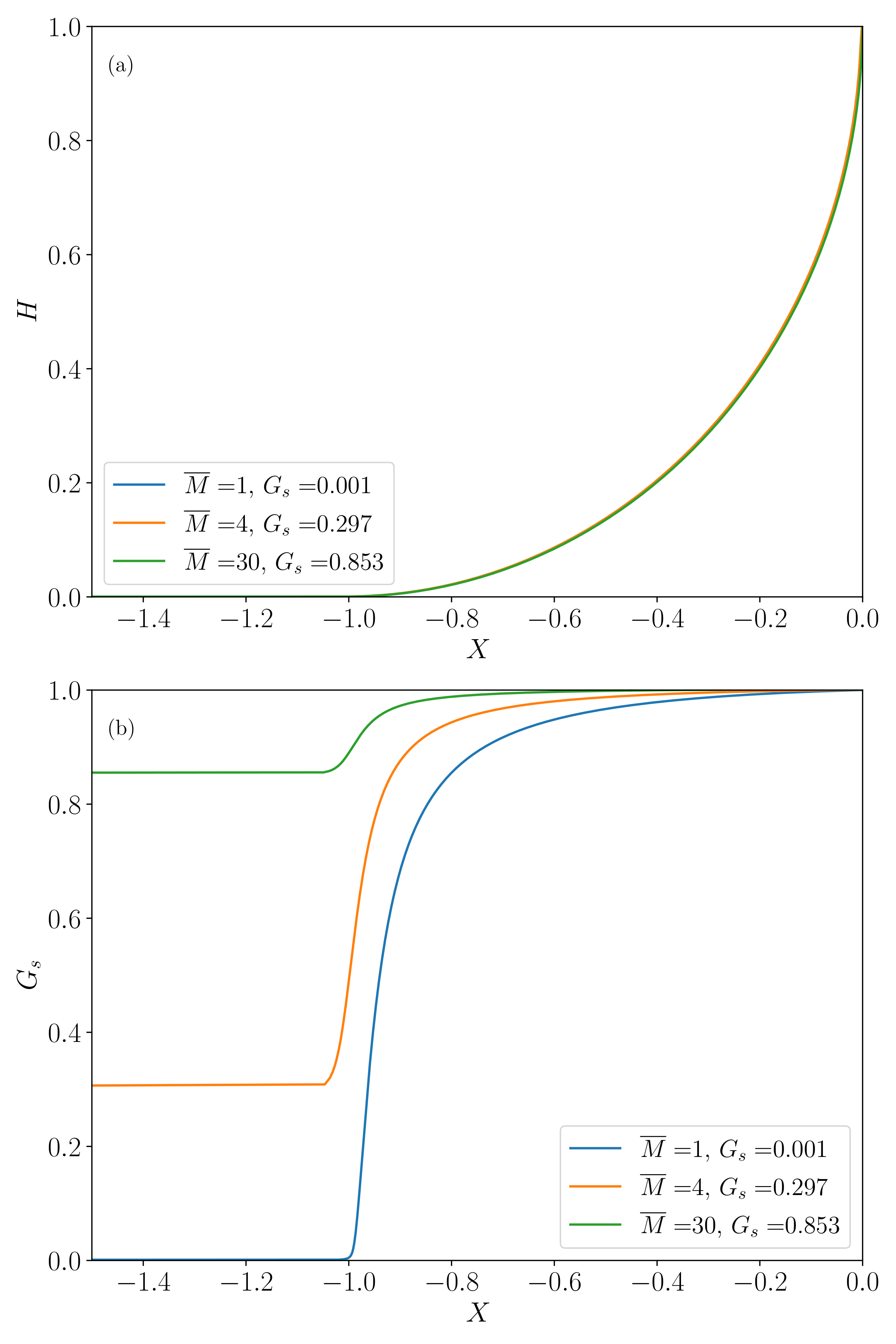
Fig. 12.2 shows numerical results, where (a) shows the film shape (not displayed in Park [Par92]) and (b) shows the normalized surfactant concentration (Fig. 5 in [Par92]). The variables here are normalized as follows:

(12.89)\[H = \frac{\overline{h}}{\overline{h}_s},~~ X = \frac{\overline{x} + s}{\overline{h}_s},~~ G = \frac{\overline{\Gamma}}{\overline{\Gamma}_f},~~ G_s = \frac{\overline{\Gamma}_s}{\overline{\Gamma}_f},~~ \overline{M} = \overline{\Gamma}_{f} M\]

Here, the overline means variables scaled with

(12.90)\[x \sim Ca^{1/3},~~ h \sim Ca^{2/3},~~ \Gamma \sim Ca^{2/3}\]

and

(12.91)\[\overline{M} = - \frac{\Gamma_f}{\mathrm{Ca}^{2/3} \, \sigma_f} \left( \frac{\partial \sigma}{\partial \Gamma} \right)_{\Gamma_f}\]

The subscript \(s\) denotes the stationary film. The subscript \(f\) denotes the front tip. The ODEs of liquid film thickness and surfactant concentration are therefore

(12.92)\[ H_{XXX} = \frac{3(H-1)}{H^3} + \frac{3\overline{M} G_X}{2H}\]
(12.93)\[ G_{X} = \frac{2(H-3)G + 4HG_s}{\overline{M} H^2 G}\]

In order to reproduce the problem with our code for the full curvature expression, we used a very small value for \(Ca_{b}\) since Park [Par92] used a simplified curvature expression (\(H_{XXX}\)). Therefore, we utilized \(Ca_{b} = 1 \times 10^{-6}\) although Park did not mention the actual value. Due to the small \(Ca_{b}\), the film thickness is extremely thin (the Bretherton scaling: \(\propto Ca_{b}^{2/3}\)). The surfactant concentration decreases from the nose toward the film because of the expansion of the surface area in the meniscus, and then it becomes constant in the film. Park [Par92] found that the film thicknening by Marangoni stress is scaled by factor of \(4^{2/3}\) at large \(\overline{M}\) [RC90].

../_images/Fig_h_g_Park.png

Fig. 12.2 Profiles of film \(H\) and surfactant concentration \(G_{s}\). This verification corresponds to Fig. 5 in Park [Par92].