Polar and axial vectors

Reference

Ando [And19]

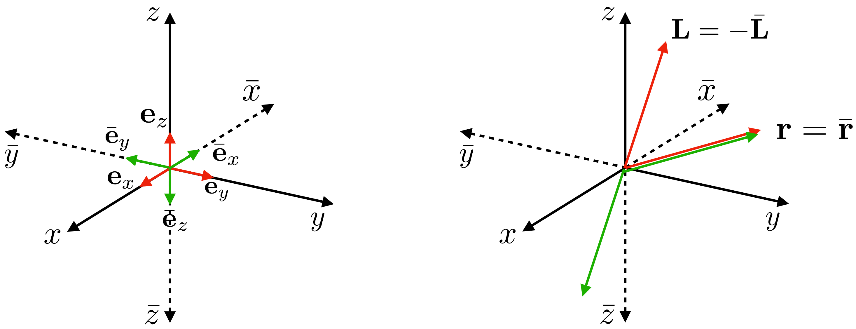
Fig. 1 Parity transformation

Polar and axial vectors are vectors characterized by their behaviors for the following parity transformation:

(12)\[\begin{split}\begin{split} &\bar{x}_{i} = - x_{i} \\ &\bar{\mathbf{e}}_{i} = - \mathbf{e}_{i} \end{split}\end{split}\]

Importantly the parity transformation changes a system from right-handed (\(x\)) to left-handed (\(\bar{x}\)), and vice versa. In the right-handed system, the cross products between the base vectors are summarized in the following matrix form:

(13)\[\begin{split}\left( \begin{array}{lll} \mathbf{e}_{x} \times \mathbf{e}_{x} &\mathbf{e}_{x} \times \mathbf{e}_{y} &\mathbf{e}_{x} \times \mathbf{e}_{z} \\ \mathbf{e}_{y} \times \mathbf{e}_{x} &\mathbf{e}_{y} \times \mathbf{e}_{y} &\mathbf{e}_{y} \times \mathbf{e}_{z} \\ \mathbf{e}_{z} \times \mathbf{e}_{x} &\mathbf{e}_{z} \times \mathbf{e}_{y} &\mathbf{e}_{z} \times \mathbf{e}_{z} \end{array} \right) = \left( \begin{array}{rrr} 0 &\mathbf{e}_{z} &-\mathbf{e}_{y} \\ -\mathbf{e}_{z} &0 &\mathbf{e}_{x} \\ \mathbf{e}_{y} &-\mathbf{e}_{x} &0 \end{array} \right)\end{split}\]

In the left-handed system, we use the left-screw law, i.e., a screw moves forward when it is rotated counterclockwise. Therefore, the cross-product rule conserves:

(14)\[\begin{split}\left( \begin{array}{lll} \bar{\mathbf{e}}_{x} \times \bar{\mathbf{e}}_{x} &\bar{\mathbf{e}}_{x} \times \bar{\mathbf{e}}_{y} &\bar{\mathbf{e}}_{x} \times \bar{\mathbf{e}}_{z} \\ \bar{\mathbf{e}}_{y} \times \bar{\mathbf{e}}_{x} &\bar{\mathbf{e}}_{y} \times \bar{\mathbf{e}}_{y} &\bar{\mathbf{e}}_{y} \times \bar{\mathbf{e}}_{z} \\ \bar{\mathbf{e}}_{z} \times \bar{\mathbf{e}}_{x} &\bar{\mathbf{e}}_{z} \times \bar{\mathbf{e}}_{y} &\bar{\mathbf{e}}_{z} \times \bar{\mathbf{e}}_{z} \end{array} \right) = \left( \begin{array}{rrr} 0 &\bar{\mathbf{e}}_{z} &-\bar{\mathbf{e}}_{y} \\ -\bar{\mathbf{e}}_{z} &0 &\bar{\mathbf{e}}_{x} \\ \bar{\mathbf{e}}_{y} &-\bar{\mathbf{e}}_{x} &0 \end{array} \right)\end{split}\]

By making use of the permutation symbol, these relations may be written as

(15)\[\begin{split}\begin{split} &\mathbf{e}_{i} = \epsilon_{ijk} \mathbf{e}_{j} \times \mathbf{e}_{k}~~~~\text{no sum on}~j, k \\ &\bar{\mathbf{e}}_{i} = \epsilon_{ijk} \bar{\mathbf{e}}_{j} \times \bar{\mathbf{e}}_{k}~~~~\text{no sum on}~j, k \end{split}\end{split}\]

or

(16)\[\begin{split}\begin{split} &\mathbf{e}_{i} \times \mathbf{e}_{j} = \epsilon_{kij} \mathbf{e}_{k} \\ &\bar{\mathbf{e}}_{i} \times \bar{\mathbf{e}}_{j} = \epsilon_{kij} \bar{\mathbf{e}}_{k} \end{split}\end{split}\]

Also

(17)\[ \epsilon_{ijk} = \mathbf{e}_{i} \cdot ( \mathbf{e}_{j} \times \mathbf{e}_{k} ) = \bar{\mathbf{e}}_{i} \cdot ( \bar{\mathbf{e}}_{j} \times \bar{\mathbf{e}}_{k} ) = \bar{\epsilon}_{ijk}\]

Then, Kronecker’s delta is the dot products between the base vectors:

(18)\[ \delta_{ij} = \mathbf{e}_{i} \cdot \mathbf{e}_{j} = \bar{\mathbf{e}}_{i} \cdot \bar{\mathbf{e}}_{j}\]

Let us begin by investigating the behavior of the position vector \(\mathbf{r}\) under the parity transformation.

(19)\[ \bar{\mathbf{r}} = \bar{x}_{i} \bar{\mathbf{e}}_{i} = ( - x_{i} ) ( - \mathbf{e}_{i} ) = x_{i} \mathbf{e}_{i} = \mathbf{r}\]

Obviously, the position vector does not change under the parity transformation. The velocity vector \(\mathbf{v}\) is the temporal derivative of \(\mathbf{r}\), i.e., \(\mathbf{v} = d \mathbf{r} / dt\). Therefore,

(20)\[ \bar{\mathbf{v}} = \frac{d \bar{\mathbf{r}}}{dt} = \frac{d \bar{x _{i}} \bar{\mathbf{e}}_{i}}{dt} = \frac{d \bar{x _{i}}}{dt} \bar{\mathbf{e}}_{i} = \left( - \frac{d x _{i}}{dt} \right) \left( - \mathbf{e}_{i} \right) = \frac{d x _{i}}{dt} \mathbf{e}_{i} = \mathbf{v}\]

The velocity vector is also unchangeable under the parity transformation. This is of course also true for the momentum vector \(\mathbf{p} = m \mathbf{v}\). Vectors unchangeable under the parity transformation are called polar vectors.

The angular momentum is given by the cross product \(\mathbf{L} = \mathbf{r} \times \mathbf{p}\). Its behavior under the parity transformation is as follows:

(21)\[ \bar{\mathbf{L}} = \bar{\mathbf{r}} \times \bar{\mathbf{p}} = \bar{x}_{i} \bar{\mathbf{e}}_{i} \times \bar{p}_{j} \bar{\mathbf{e}}_{j} = \bar{x}_{i} \bar{p}_{j} \bar{\mathbf{e}}_{i} \times \bar{\mathbf{e}}_{j} = (- x_{i} ) (- p_{j}) \bar{\mathbf{e}}_{i} \times \bar{\mathbf{e}}_{j} = x_{i} p_{j} \bar{\mathbf{e}}_{i} \times \bar{\mathbf{e}}_{j}\]

where the components were transformed using the polar character. Then,

(22)\[ x_{i} p_{j} \bar{\mathbf{e}}_{i} \times \bar{\mathbf{e}}_{j} = \epsilon_{kij} x_{i} p_{j} \bar{\mathbf{e}}_{k} = - \epsilon_{kij} x_{i} p_{j} \mathbf{e}_{k} = - \mathbf{L}\]

Thus, \(\bar{\mathbf{L}} = - \mathbf{L}\). This result clearly shows that the parity transformation changes the direction of the angular momentum. It should however be noted that the direction of rotation represented by \(\mathbf{L}\) does not change. For example, for a point mass rotating counterclockwise about the \(z\) axis on the \(xy\) plane, \(\mathbf{L}\) directs the positive \(z\). In the left-handed system \(\bar{x}\) obtained by the parity transformation, \(\bar{\mathbf{L}} = - \mathbf{L}\), so that the direction of \(\bar{\mathbf{L}}\) is the negative \(z\). This vector also represents the counterclockwise rotation on the \(xy\) plane since the left-screw law is applied in the \(\bar{x}\) system. Therefore, the reversal of \(\mathbf{L}\) is required to maintain the physical state of the rotation. Vectors possessing this character are axial vectors (or pseudo vectors).

The differential operator \(\nabla\) is a vector-like operator written by

(23)\[ \nabla = \frac{\partial}{\partial x_{i}} \mathbf{e}_{i}\]

This can be regarded as polar vector as shown below:

(24)\[ \bar{\nabla} = \frac{\partial}{\partial \bar{x}_{i}} \bar{\mathbf{e}}_{i} = \left( - \frac{\partial}{\partial x_{i}} \right) \left( - \mathbf{e}_{i} \right) = \frac{\partial}{\partial x_{i}} \mathbf{e}_{i} = \nabla\]

The vorticity defined by

(25)\[ \boldsymbol{\omega} = \nabla \times \mathbf{v}\]

is an axial vector as demonstrated below

(26)\[ \bar{\boldsymbol{\omega}} = \bar{\nabla} \times \bar{ \mathbf{v} } = \epsilon_{ijk} \frac{\partial \bar{v}_{k}}{\partial \bar{x}_{j}} \bar{\mathbf{e}}_{i} = - \epsilon_{ijk} \frac{\partial v_{k}}{\partial x_{j}} \mathbf{e}_{i} = - \nabla \times \mathbf{v} = - \boldsymbol{\omega}\]

It is obvious that polar vectors cannot be added to axial vectors since their behaviors under the transformation are different. In the equation of motion of fluids, we see

(27)\[ \frac{\partial \mathbf{v}}{\partial t} + \nabla \left( \frac{v^{2}}{2} \right) + \boldsymbol{\omega} \times \mathbf{v} = - \frac{\nabla p}{\rho}\]

The first term is polar vector. The second term is also polar due to the polar nature of \(\nabla\). Therefore, the third term must also be polar vector, showing that the cross product between an axial vector and a polar vector generates a polar vector. Let us develop lookup tables for the results of cross and dot products between vectors. In the following the superscripts \((p)\) and \((a)\) denote polar and axial vectors, respectively. First, the cross product \(\mathbf{A}\) between polar vectors \(\mathbf{a}^{(p)}\) and \(\mathbf{b}^{(p)}\) is

(28)\[ \bar{ \mathbf{A} } = \bar{ \mathbf{a} }^{(p)} \times \bar{ \mathbf{b} }^{(p)} = \epsilon_{ijk} \bar{a}_{j} \bar{b}_{k} \bar{\mathbf{e}}_{i} = - \epsilon_{ijk} a_{j} b_{k} \mathbf{e}_{i} = - \mathbf{a}^{(p)} \times \mathbf{b}^{(p)} = - \mathbf{A}~~~~(\text{axial vector})\]

(29)\[\begin{split}\begin{split} \bar{ \mathbf{A} } &= \bar{ \mathbf{a} }^{(a)} \times \bar{ \mathbf{b} }^{(a)} = ( \bar{a}^{(a)}_{i} \bar{\mathbf{e}}_{i}) \times ( \bar{b}^{(a)}_{j} \bar{\mathbf{e}}_{j} ) = ( a^{(a)}_{i} \bar{\mathbf{e}}_{i}) \times ( b^{(a)}_{j} \bar{\mathbf{e}}_{j} ) = a^{(a)}_{i} b^{(a)}_{j} \bar{\mathbf{e}}_{i} \times \bar{\mathbf{e}}_{j} \\ &= \epsilon_{kij} a^{(a)}_{i} b^{(a)}_{j} \bar{\mathbf{e}}_{k} = - \epsilon_{kij} a^{(a)}_{i} b^{(a)}_{j} \mathbf{e}_{k} = - \mathbf{a}^{(a)} \times \mathbf{b}^{(a)} = - \mathbf{A}~~~~(\text{axial vector}) \end{split}\end{split}\]

where we used the inversion of the components of the axial vector: \(\bar{a}^{(a)}_{i} \bar{\mathbf{e}}_{i} = a^{(a)}_{i} \bar{\mathbf{e}}_{i}\). Then,

(30)\[\begin{split}\begin{split} \bar{ \mathbf{A} } &= \bar{ \mathbf{a} }^{(p)} \times \bar{ \mathbf{b} }^{(a)} = ( \bar{a}^{(p)}_{i} \bar{\mathbf{e}}_{i}) \times ( \bar{b}^{(a)}_{j} \bar{\mathbf{e}}_{j} ) = ( - a^{(p)}_{i} \bar{\mathbf{e}}_{i}) \times ( b^{(a)}_{j} \bar{\mathbf{e}}_{j} ) = - a^{(p)}_{i} b^{(a)}_{j} \bar{\mathbf{e}}_{i} \times \bar{\mathbf{e}}_{j} \\ &= - \epsilon_{kij} a^{(p)}_{i} b^{(a)}_{j} \bar{\mathbf{e}}_{k} = \epsilon_{kij} a^{(p)}_{i} b^{(a)}_{j} \mathbf{e}_{k} = \mathbf{a}^{(p)} \times \mathbf{b}^{(a)} = \mathbf{A}~~~~(\text{polar vector}) \end{split}\end{split}\]

(31)\[\begin{split}\begin{split} \bar{ \mathbf{A} } &= \bar{ \mathbf{a} }^{(a)} \times \bar{ \mathbf{b} }^{(p)} = ( \bar{a}^{(a)}_{i} \bar{\mathbf{e}}_{i}) \times ( \bar{b}^{(p)}_{j} \bar{\mathbf{e}}_{j} ) = ( a^{(a)}_{i} \bar{\mathbf{e}}_{i}) \times ( - b^{(p)}_{j} \bar{\mathbf{e}}_{j} ) = - a^{(a)}_{i} b^{(p)}_{j} \bar{\mathbf{e}}_{i} \times \bar{\mathbf{e}}_{j} \\ &= - \epsilon_{kij} a^{(a)}_{i} b^{(p)}_{j} \bar{\mathbf{e}}_{k} = \epsilon_{kij} a^{(a)}_{i} b^{(p)}_{j} \mathbf{e}_{k} = \mathbf{a}^{(a)} \times \mathbf{b}^{(p)} = \mathbf{A}~~~~(\text{polar vector}) \end{split}\end{split}\]

Types of scalars generated by dot products are as follows.

(32)\[ \bar{\alpha} = \bar{\mathbf{a}}^{(p)} \cdot \bar{\mathbf{b}}^{(p)} = \bar{a}^{(p)}_{i} \bar{\mathbf{e}}_{i} \cdot \bar{b}^{(p)}_{j} \bar{\mathbf{e}}_{j} = \bar{a}^{(p)}_{i} \bar{b}^{(p)}_{j} \delta_{ij} = \bar{a}^{(p)}_{i} \bar{b}^{(p)}_{i} = (-a^{(p)}_{i}) (-b^{(p)}_{i}) = a^{(p)}_{i} b^{(p)}_{i} = \alpha~~~~(\text{scalar})\]

(33)\[ \bar{\alpha} = \bar{\mathbf{a}}^{(a)} \cdot \bar{\mathbf{b}}^{(a)} = \bar{a}^{(a)}_{i} \bar{\mathbf{e}}_{i} \cdot \bar{b}^{(a)}_{j} \bar{\mathbf{e}}_{j} = a^{(a)}_{i} \bar{\mathbf{e}}_{i} \cdot b^{(a)}_{j} \bar{\mathbf{e}}_{j} = a^{(a)}_{i} b^{(a)}_{j} \delta_{ij} = a^{(a)}_{i} b^{(a)}_{i} = \alpha~~~~(\text{scalar})\]

(34)\[ \bar{\alpha} = \bar{\mathbf{a}}^{(p)} \cdot \bar{\mathbf{b}}^{(a)} = \bar{a}^{(p)}_{i} \bar{\mathbf{e}}_{i} \cdot \bar{b}^{(a)}_{j} \bar{\mathbf{e}}_{j} = -a^{(p)}_{i} b^{(a)}_{j} \delta_{ij} = -a^{(p)}_{i} b^{(a)}_{i} = -\alpha~~~~(\text{pseudo scalar})\]

(35)\[ \bar{\alpha} = \bar{\mathbf{a}}^{(a)} \cdot \bar{\mathbf{b}}^{(p)} = \bar{a}^{(a)}_{i} \bar{\mathbf{e}}_{i} \cdot \bar{b}^{(p)}_{j} \bar{\mathbf{e}}_{j} = -a^{(a)}_{i} b^{(p)}_{j} \delta_{ij} = -a^{(a)}_{i} b^{(p)}_{i} = -\alpha~~~~(\text{pseudo scalar})\]

For the cross product:

	polar	axial
polar	axial	polar
axial	polar	axial

For the dot product:

	polar	axial
polar	scalar	pseudo scalar
axial	pseudo scalar	scalar

In the discussion on the Stokes drag, we set

(36)\[ \mathbf{v} = \nabla \times \mathbf{A} + \mathbf{u}\]

where \(\mathbf{v}\) and \(\mathbf{u}\) are polar vectors. Therefore, \(\nabla \times \mathbf{A}\) should also be polar to add them each other. As we discussed \(\nabla\) behaves like polar vector, so that, \(\mathbf{A}\) should be an axial vector. The vector potential \(\mathbf{A}\) obviously depends on \(\mathbf{u}\) and should be proportional to \(\mathbf{u}\) since \(\nabla \times \mathbf{A}\) needs to produce \(- \mathbf{u}\) at the sphere surface to satisfy the boundary condition \(\mathbf{v} = 0\) at \(r = a\). On the other hand, the vector potential should also be a function of \(\mathbf{r}\). The velocity and position vectors are polar vectors. Therefore, \(\mathbf{r} \times \mathbf{u}\) is only the form satisfying all the requirements for \(\mathbf{A}\). Thus,

(37)\[ \mathbf{A} = g(r) \mathbf{e}_{r} \times \mathbf{u}\]