8.2. Drag acting on a fluid sphere in Stokes flow

Summary

• Subject: Hadamard-Rybczynski drag [Had11]

• Main conclusion: Drag is a function of fluids viscosities, \(F_{D} = \left( \frac{2 \mu^{(e)} + 3 \mu^{(i)}}{\mu^{(e)} + \mu^{(i)}} \right) 2 \pi \mu^{(e)} u a\).

• Key idea Boundary conditions at fluids interface; in particular, continuity of tangential viscous stresses at interface between two fluids connects the two velocity fields.

• Reference: Derivation presented here is given by Landau and Lifshitz [LL87] (Chap. 2). Recommended to read the textbook to follow the theory.

A fluid sphere of viscosity \(\mu^{(i)}\) is fixed in a uniform flow of \(\mu^{(e)}\), where the superscripts \((i)\) and \((e)\) denote the internal and external fluids, respectively. The fluids are Newtonian and the Reynolds number is small. Therefore, the flow field in the external fluid can be obtained in the same manner for the Stokes drag, that is,

(8.69)\[ \mathbf{v}^{(e)} = \mathbf{u} - \alpha \frac{\mathbf{u} + (\mathbf{u} \cdot \mathbf{e}_{r}) \mathbf{e}_{r}}{r} + \beta \frac{ 3 (\mathbf{u} \cdot \mathbf{e}_{r}) \mathbf{e}_{r} - \mathbf{u}}{r^{3}}\]

Note that the coefficients \(\alpha\) and \(\beta\) have values different from those for the Stokes drag as will be discussed later. For the internal flow, we assume the velocity in the form \(\mathbf{v}^{(i)} = \nabla \times \mathbf{A} = \nabla \times \nabla \times f \mathbf{u}\). We do not need to put \(\mathbf{u}\) on the R.H.S. since the internal flow does not require the far field boundary condition. Then, the procedure is the same with Drag acting on a solid sphere in Stokes flow (LL) up to

(8.70)\[ \nabla^{2} \nabla^{2} f = \text{const.}\]

For the external flow, the constant on the R.H.S. could be set as zero because of the far field boundary condition \(\mathbf{v}^{(e)} \rightarrow \mathbf{u}\). However, we need to keep it for the internal velocity field. The equation for \(f\) is therefore,

(8.71)\[ \frac{1}{r^{2}} \frac{d}{dr} \left\{ r^{2} \frac{d}{dr} \left( \frac{1}{r^{2}} \frac{d}{dr} \left( r^{2} \frac{df}{dr} \right) \right) \right\} = b_{0}\]

Integrating this ODE yields

(8.72)\[ f = \frac{b_{0}}{120} r^{4} - \frac{b_{1}}{2} r + \frac{b_{2}}{6} r^{2} - \frac{b_{3}}{r} + b_{4}\]

The constant \(b_{4}\) can be safely omitted. Rewriting the constants gives

(8.73)\[ f = \hat{\alpha} r + \frac{\hat{\beta}}{r} + \delta r^{2} + \gamma r^{4}\]

However, \(\hat{\alpha}\) and \(\hat{\beta}\) must be zero to have \(\mathbf{v}^{(i)}\) finite at the origin (\(r = 0\)).

As we have already seen, the functional form \(\alpha r\) in \(f\) yields the factor of \(1/r\) in \(\mathbf{v}\). \(\nabla \times \nabla \times f \mathbf{u} = \nabla \nabla \cdot f \mathbf{u} - \nabla^{2} f \mathbf{u} \rightarrow \frac{\partial}{\partial x_{i}} \frac{\partial fu_{j}}{\partial x_{j}} - \frac{\partial^{2} f u_{i}}{\partial x_{j} \partial x_{j}} = u_{j} \frac{\partial}{\partial x_{i}} \frac{\partial f}{\partial x_{j}} - u_{i} \frac{\partial^{2} f}{\partial x_{j} \partial x_{j}}\)

The term proportional to \(r\) becomes \(u_{j} \frac{\partial}{\partial x_{i}} \frac{\partial r}{\partial x_{j}} - u_{i} \frac{\partial^{2} r}{\partial x_{j} \partial x_{j}} = u_{j} \frac{\partial}{\partial x_{i}} \frac{x_{j}}{r} - u_{i} \frac{\partial }{\partial x_{j}} \frac{x_{j}}{r} = \frac{u_{i}}{r} - \frac{u_{j} x_{j} x_{i}}{r^{3}} - \frac{3 u_{i}}{r} + \frac{u_{i} x_{j} x_{j}}{r^{3}} = - \frac{u_{j} x_{j} x_{i}}{r^{3}} - \frac{u_{i}}{r}\)

Therefore,

(8.74)\[ f = \delta r^{2} + \gamma r^{4}\]

By substituting this expression into the velocity equation we have

(8.75)\[ \mathbf{v}^{(i)} = \nabla \times \nabla \times ( f \mathbf{u} ) = \nabla \times \nabla \times { (\gamma r^{4} + \delta r^{2}) \mathbf{u} }\]

Expanding this equation in the component form as

(8.76)\[\begin{split}\begin{split} \nabla \times \nabla \times ( f \mathbf{u} ) &= \nabla \nabla \cdot f \mathbf{u} - \nabla^{2} f \mathbf{u} \rightarrow \frac{\partial }{\partial x_{i}} \frac{\partial f u_{j}}{\partial x_{j}} - \frac{\partial^{2} f u_{i}}{\partial x_{j} \partial x_{j}} \\ &= u_{j} \frac{\partial^{2} f}{\partial x_{i} \partial x_{j}} - u_{i} \frac{\partial^{2} f }{\partial x_{j} \partial x_{j}} \\ &= \left(u_{j} \frac{\partial }{\partial x_{i}} - u_{i} \frac{\partial }{\partial x_{j}} \right) \frac{\partial f}{\partial x_{j}} \end{split}\end{split}\]

The gradient of \(f\) is

(8.77)\[ \frac{\partial f}{\partial x_{j}} = \frac{\partial (\gamma r^{4} + \delta r^{2})}{\partial x_{j}} = ( 4 \gamma r^{2} + 2 \delta ) x_{j}\]

Further differentiating this result gives

(8.78)\[\begin{split}\begin{split} &\frac{\partial}{\partial x_{i}} ( 4 \gamma r^{2} + 2 \delta ) x_{j} = 8 \gamma x_{i} x_{j} + ( 4 \gamma r^{2} + 2 \delta ) \delta_{ij} \\ &\frac{\partial}{\partial x_{j}} ( 4 \gamma r^{2} + 2 \delta ) x_{j} = 8 \gamma x_{j} x_{j} + 2 ( 2 \gamma r^{2} + \delta ) \delta_{jj} = 20 \gamma r^{2} + 6 \delta \end{split}\end{split}\]

Substituting these results into Eq. (8.76) yields

(8.79)\[\begin{split}\begin{split} \left(u_{j} \frac{\partial }{\partial x_{i}} - u_{i} \frac{\partial }{\partial x_{j}} \right) \frac{\partial f}{\partial x_{j}} &= u_{j} ( 8 \gamma x_{i} x_{j} + ( 4 \gamma r^{2} + 2 \delta ) \delta_{ij} ) - u_{i} ( 20 \gamma r^{2} + 6 \delta ) \\ &= \gamma r^{2} \left( \frac{8 u_{j} x_{j} x_{i}}{r^{2}} - 16 u_{i} \right) - 4 \delta u_{i} \end{split}\end{split}\]

Recasting the constants as \(\delta = A/4\) and \(\gamma = B/8\) gives

(8.80)\[ \gamma r^{2} \left( \frac{8 u_{j} x_{j} x_{i}}{r^{2}} - 16 u_{i} \right) - 4 \delta u_{i} = B r^{2} \left( \frac{u_{j} x_{j} x_{i}}{r^{2}} - 2 u_{i} \right) - A u_{i}\]

Thus,

(8.81)\[ \mathbf{v}^{(i)} = - A \mathbf{u} + B r^{2} \left( ( \mathbf{u} \cdot \mathbf{e}_{r} ) \mathbf{e}_{r} - 2 \mathbf{u} \right)\]

The constants \(\alpha\), \(\beta\), \(A\) and \(B\) are determined by the boundary conditions for the velocities and the viscous stresses. The components of \(\mathbf{v}^{(e)}\) are

(8.82)\[\begin{split}\begin{split} &v_{r}^{(e)} = \mathbf{v}^{(e)} \cdot \mathbf{e}_{r} = - u \cos \theta \left( 1 - \frac{2 \alpha}{r} + \frac{2 \beta}{r^{3}} \right) \\ &v_{\theta}^{(e)} = \mathbf{v}^{(e)} \cdot \mathbf{e}_{\theta} = u \sin \theta \left( 1 - \frac{\alpha}{r} - \frac{\beta}{r^{3}} \right) \end{split}\end{split}\]

In the internal fluid,

(8.83)\[\begin{split}\begin{split} &v_{r}^{(i)} = \mathbf{v}^{(i)} \cdot \mathbf{e}_{r} = - u \cos \theta \left( - A - B r^{2} \right) \\ &v_{\theta}^{(i)} = \mathbf{v}^{(i)} \cdot \mathbf{e}_{\theta} = u \sin \theta \left( - A - 2 B r^{2} \right) \end{split}\end{split}\]

The \(r \theta\) components of the viscous stress

(8.84)\[ \tau_{r \theta} = \mu \left( \frac{1}{r} \frac{\partial v_{r}}{\partial \theta} + \frac{\partial v_{\theta}}{\partial r} - \frac{v_{\theta}}{r} \right)\]

are

(8.85)\[\begin{split}\begin{split} &\tau_{r \theta}^{(e)} = \beta \frac{6 \mu^{(e)} u}{r^{4}} \sin \theta \\ &\tau_{r \theta}^{(i)} = - 3 B \mu^{(i)} r u \sin \theta \end{split}\end{split}\]

At the interface, they are

(8.86)\[\begin{split}\begin{split} \left. v_{r}^{(e)} \right|_{r=a} &= - u \cos \theta \left( 1 - \frac{2 \alpha}{a} + \frac{2 \beta}{a^{3}} \right) \\ \left. v_{\theta}^{(e)} \right|_{r=a} &= u \sin \theta \left( 1 - \frac{\alpha}{a} - \frac{\beta}{a^{3}} \right) \\ \left. v_{r}^{(i)} \right|_{r=a} &= - u \cos \theta \left( - A - B a^{2} \right) \\ \left. v_{\theta}^{(i)} \right|_{r=a} &= u \sin \theta \left( - A - 2 B a^{2} \right) \\ \left. \tau_{r \theta}^{(e)} \right|_{r=a} &= \beta \frac{6 \mu^{(e)} u}{a^{4}} \sin \theta \\ \left. \tau_{r \theta}^{(i)} \right|_{r=a} &= - 3 B \mu^{(i)} a u \sin \theta \end{split}\end{split}\]

The boundary conditions are

• The velocity normal to the interface is continuous and is zero because the sphere is motionless: \(\left. v_{r}^{(e)} \right|_{r=a} = \left. v_{r}^{(i)} \right|_{r=a} = 0\)

• The velocity tangent to the interface is continuous: \(\left. v_{\theta}^{(e)} \right|_{r=a} = \left. v_{\theta}^{(i)} \right|_{r=a}\)

• The tangential viscous stress is continuous: \(\left. \tau_{r \theta}^{(e)} \right|_{r=a} = \left. \tau_{r \theta}^{(i)} \right|_{r=a}\)

Applying the boundary conditions yields the following simultaneous equations for the constants:

(8.87)\[\begin{split}\begin{split} &A + a^{2} B = 0 \\ &- 2 a^{2} \alpha + 2 \beta + a^{3} = 0 \\ &a^{3} A + 2 a^{5} B - a^{2} \alpha - \beta + a^{3} = 0 \\ &\mu^{(i)} a^{5} B + 2 \mu^{(e)} \beta = 0 \end{split}\end{split}\]

From the second equation, \(\alpha = a/2 + \beta/a^{2}\). Substituting this and the first equation into the third equation gives \(B = 2 \beta / a^{5} - 1/2a^{2}\). By substituting the fourth equation into the R.H.S. we obtain \(B\), and then, \(\beta\) can be obtained from the fourth equation by using \(B\). Thus,

(8.88)\[\begin{split}\begin{split} &\alpha = \frac{a}{4} \frac{2 \mu^{(e)} + 3 \mu^{(i)}}{\mu^{(e)} + \mu^{(i)}} \\ &\beta = \frac{a^{3}}{4} \frac{\mu^{(i)}}{\mu^{(e)} + \mu^{(i)}} \\ &A = \frac{1}{2} \frac{\mu^{(e)}}{\mu^{(e)} + \mu^{(i)}} \\ &B = - \frac{1}{2 a^{2}} \frac{\mu^{(e)}}{\mu^{(e)} + \mu^{(i)}} \end{split}\end{split}\]

The stream functions are given by

(8.89)\[\begin{split}\begin{split} &\psi^{(e)} = -\frac{u r^{2} \sin^{2} \theta}{2} \left\{ 1 - \frac{2 \alpha}{r} + \frac{2 \beta}{r^{3}} \right\} \\ &\psi^{(i)} = \frac{u r^{2} \sin^{2} \theta}{2} \left\{ A + B r^{2} \right\} \end{split}\end{split}\]

where the velocity components are deduced from \(\psi\) as

(8.90)\[\begin{split}\begin{split} &v_{r} = \frac{1}{r^{2} \sin \theta} \frac{\partial \psi}{\partial \theta} \\ &v_{\theta} = - \frac{1}{r \sin \theta} \frac{\partial \psi}{\partial r} \end{split}\end{split}\]

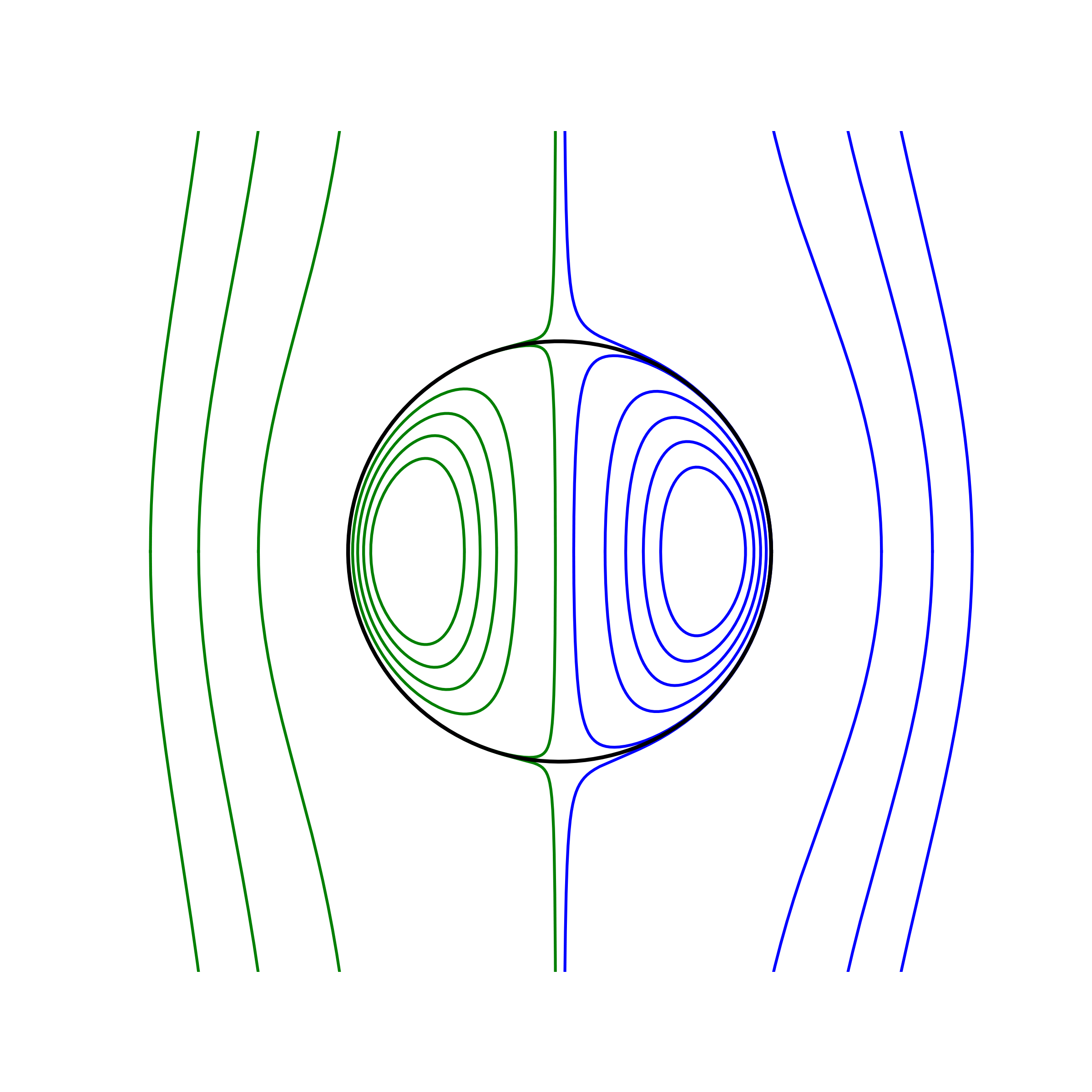
Fig. 8.4 shows several streamlines for \(\psi\).

Fig. 8.4 Flow in/about fluid sphere. (left) \(\mu^{(i)}/\mu^{(e)} = 0\), \(\psi^{(e)} \sim 0, = -0.3, -0.6, -0.9\), \(\psi^{(i)} \sim 0, = 0.01, 0.02, 0.04\). (right) \(\mu^{(i)}/\mu^{(e)} = 10\), \(\psi^{(e)} \sim 0, = -0.2, -0.4, -0.6\), \(\psi^{(i)} \sim 0, = 0.001, 0.002, 0.003, 0.004\).

Let us calculate \(\tau_{rr}\) and the pressure to obtain the drag coefficient. The viscous stress is

(8.91)\[ \tau_{rr}^{(e)} = 2 \mu \frac{\partial v_{r}}{\partial r} = - 4 \mu u \cos \theta \left( \frac{\alpha}{r^{2}} - \frac{3 \beta}{r^{4}} \right)\]

and at the interface

(8.92)\[ \left. \tau_{rr}^{(e)} \right|_{r=a} = - 4 \mu u \cos \theta \left( \frac{\alpha}{a^{2}} - \frac{3 \beta}{a^{4}} \right)\]

The pressure can be obtained using the same manner for the Stokes flow, so that

(8.93)\[ p^{(e)} = p_{0} - \frac{2 \alpha \mu^{(e)} (\mathbf{u} \cdot \mathbf{e}_{r})}{r^{2}}\]

The pressure at the interface is given by

(8.94)\[ \left. p^{(e)} \right|_{r=a} = p_{0} + \frac{2 \alpha \mu^{(e)} u \cos \theta}{a^{2}}\]

By substituting the stress components into

(8.95)\[ F_{D} = \iint_{S} (p \cos \theta - \tau_{rr} \cos \theta + \tau_{\theta r} \sin \theta) dS\]

we have

(8.96)\[\begin{split}\begin{split} F_{D} &= 2 \pi a^{2} \int_{0}^{\pi} \left( \frac{2 \alpha \mu^{(e)} u}{a^{2}} \cos^{2} \theta + 4 \mu u \left( \frac{\alpha}{a^{2}} - \frac{3 \beta}{a^{4}} \right) \cos^{2} \theta + \beta \frac{6 \mu^{(e)} u}{a^{4}} \sin^{2} \theta \right) \sin \theta d\theta \\ &= 4 \pi \mu^{(e)} u \left\{ \left( 3 \alpha - \frac{6 \beta}{a^{2}} \right) \int_{0}^{\pi} \cos^{2} \theta \sin \theta d\theta + \frac{3 \beta}{a^{2}} \int_{0}^{\pi} \sin^{3} \theta d\theta \right\} \\ \end{split}\end{split}\]

The first and second integrals are \(2/3\) and \(4/3\), respectively, yielding

(8.97)\[ F_{D} = 8 \pi \mu^{(e)} u \alpha = \left( \frac{2 \mu^{(e)} + 3 \mu^{(i)}}{\mu^{(e)} + \mu^{(i)}} \right) 2 \pi \mu^{(e)} u a\]

By defining the Reynolds number and the drag coefficient as

(8.98)\[ Re = \frac{2 \rho^{(e)} u a}{\mu^{(e)}}\]

and

(8.99)\[ C_{D} = \frac{F_{D}}{\frac{1}{2} \rho^{(e)} u^{2} \pi a^{2}}\]

we obtain

(8.100)\[ C_{D} = \frac{8}{Re} \left( \frac{2 \mu^{(e)} + 3 \mu^{(i)}}{\mu^{(e)} + \mu^{(i)}} \right)\]

The flow is known as the Hadamard-Rybczynski solution. In the limiting case of \(\mu^{(i)}/\mu^{(e)} \rightarrow \infty\), the drag coefficient becomes

(8.101)\[ C_{D} \rightarrow \frac{24}{Re}\]

which corresponds to that of the Stokes solution. On the other hand, \(\mu^{(i)}/\mu^{(e)} \rightarrow 0\) yields

(8.102)\[ C_{D} \rightarrow \frac{16}{Re}\]

Bubbles of small Reynolds numbers show to have this drag coefficient.