Biot-Savart law

Referred from

Lift acting on spherical body in inviscid flow with weak shear

References

Saffman [Saf95]

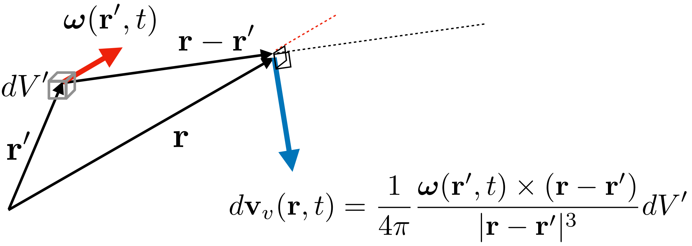
Fig. 2 Biot-Savart law

Let us consider the following conditions for a rotational flow: \begin{enumerate} \item The velocity field, \(\mathbf{v}\), satisfies \(\nabla \cdot \mathbf{v} = 0\). \item The fluid region is singly connected. \item The normal component, \(\mathbf{n} \cdot \mathbf{v}\), of the velocity is given at all bounding surfaces \(S\). \item The velocity \(\mathbf{v}\) vanishes at infinity when the fluid is unbounded. \item The normal component, \(\mathbf{n} \cdot \boldsymbol{\omega}\), of vorticity vanishes on \(S\). \item The vorticity field \(\boldsymbol{\omega}\) is compact when the fluid is unbounded. \end{enumerate} The velocity field under these conditions can be expressed as the sum of a solenoidal velocity potential component, \(\mathbf{v}_{v}\), for which \(\nabla \cdot \mathbf{v}_{v} = 0\), and an irrotational scalar component, \(\nabla \phi\), i.e.,

(38)\[ \mathbf{v} (\mathbf{r}, t) = \mathbf{v}_{v} (\mathbf{r}, t) + \nabla \phi\]

where the irrotational component is determined by the Poisson equation:

(39)\[ \nabla^{2} \phi = 0\]

with the boundary condition

(40)\[ \mathbf{n} \cdot \nabla \phi = \mathbf{n} \cdot \mathbf{v} - \mathbf{n} \cdot \mathbf{v}_{v}\]

or

(41)\[ \phi \rightarrow 0~~~~\text{as}~r \rightarrow \infty\]

when the fluid is unbounded. Taking \(rot\) of Eq. (38) yields

(42)\[ \nabla \times \mathbf{v}_{v} = \boldsymbol{\omega}\]

since \(\nabla \times \nabla \phi = 0\). The solenoidal component is constructed by the vorticity distribution (\ref{Auton_Auton-BiotSavart})

(43)\[ \mathbf{v}_{v} (\mathbf{r}, t) = \frac{1}{4 \pi} \iiint_{V'} \frac{\boldsymbol{\omega} (\mathbf{r}', t) \times (\mathbf{r} - \mathbf{r}') }{| \mathbf{r} - \mathbf{r}' |^{3}} dV'\]

where \(\mathbf{r}' = (x', y', z')\) and \(dV' = dx' dy' dz'\). This is analogous to the relation between a electric current density and a magnetic flux field. Eq. (43) is therefore called the Biot-Savart law for the fluid velocity induced by the vorticity distribution. Since

(44)\[ \frac{\partial }{\partial x_{k}} \frac{1}{| \mathbf{r}' - \mathbf{r} |} = \frac{x'_{k} - x_{k}}{| \mathbf{r}' - \mathbf{r} |^{3}}\]

we can rewrite Eq. (43) in the following form

(45)\[ \mathbf{v}_{v} (\mathbf{r}, t) = - \frac{1}{4 \pi} \iiint_{V'} \boldsymbol{\omega} (\mathbf{r}', t) \times \nabla \frac{1}{| \mathbf{r}' - \mathbf{r} |} dV'\]

Let us see the Biot-Savart velocity field satisfies \(\nabla \cdot \mathbf{v}_{v} = 0\) and \(\nabla \times \mathbf{v}_{v} = \boldsymbol{\omega}\) in the following. For simplicity, we write \(\boldsymbol{\omega}' = \boldsymbol{\omega} (\mathbf{r}', t)\), \(\nabla' = \partial / \partial \mathbf{r}'\) and \(r = | \mathbf{r} - \mathbf{r}' |\). Taking \(div\) of Eq. (45) we have

(46)\[ \nabla \cdot \mathbf{v}_{v} = - \frac{1}{4 \pi} \nabla \cdot \iiint_{V'} \boldsymbol{\omega}' \times \nabla \frac{1}{r} dV' = - \frac{1}{4 \pi} \iiint_{V'} \nabla \cdot \left( \boldsymbol{\omega}' \times \nabla \frac{1}{r} \right) dV' \]

We can take \(\boldsymbol{\omega}'\) out from the divergence since it is a function of \(\mathbf{r}'\), not \(\mathbf{r}\). Therefore,

\(- \nabla \cdot \left( \boldsymbol{\omega}' \times \nabla \frac{1}{r} \right) \rightarrow - \frac{\partial }{\partial x_{k}} \left( \epsilon_{kij} \omega'_{i} \frac{\partial }{\partial x_{j}} \frac{1}{r} \right) = - \omega'_{i} \epsilon_{kij} \frac{\partial }{\partial x_{k}} \left( \frac{\partial }{\partial x_{j}} \frac{1}{r} \right)\) \(= \omega'_{i} \epsilon_{ikj} \frac{\partial }{\partial x_{k}} \left( \frac{\partial }{\partial x_{j}} \frac{1}{r} \right) \rightarrow \boldsymbol{\omega}' \cdot \left( \nabla \times \nabla \frac{1}{r} \right)\)

(47)\[ \nabla \cdot \mathbf{v}_{v} = \frac{1}{4 \pi} \iiint_{V'} \boldsymbol{\omega}' \cdot \left( \nabla \times \nabla \frac{1}{r} \right) dV' \]

However, because of the identity \(\nabla \times \nabla~\text{(any scalar)} = 0\),

(48)\[ \nabla \cdot \mathbf{v}_{v} = 0\]

The Biot-Savart velocity field is thus confirmed to be solenoidal. Then, we take \(rot\) of Eq. (45):\footnote{

(49)\[\begin{split}\begin{split} - \nabla \times \iiint_{V'} \boldsymbol{\omega}' \times \nabla \frac{1}{r} &\rightarrow - \epsilon_{ijk} \frac{\partial}{\partial x_{j}} \epsilon_{kmn} \omega'_{m} \frac{\partial}{\partial x_{n}} \frac{1}{r} = - \epsilon_{ijk} \epsilon_{kmn} \omega'_{m} \frac{\partial}{\partial x_{j}} \frac{\partial}{\partial x_{n}} \frac{1}{r} \\ &= - (\delta_{im} \delta_{jn} - \delta_{in} \delta_{jm}) \omega'_{m} \frac{\partial}{\partial x_{j}} \frac{\partial}{\partial x_{n}} \frac{1}{r} = - \omega'_{i} \frac{\partial}{\partial x_{j}} \frac{\partial}{\partial x_{j}} \frac{1}{r} + \omega'_{j} \frac{\partial}{\partial x_{j}} \frac{\partial}{\partial x_{i}} \frac{1}{r} \\ &\rightarrow - \boldsymbol{\omega}' \nabla^{2} (1/r) + \boldsymbol{\omega} \cdot \nabla \nabla (1/r) \end{split}\end{split}\]

}

(50)\[ \nabla \times \mathbf{v}_{v} = - \frac{1}{4 \pi} \nabla \times \iiint_{V'} \boldsymbol{\omega}' \times \nabla \frac{1}{r} dV' = \frac{1}{4 \pi} \iiint_{V'} \left\{ - \boldsymbol{\omega}' \nabla^{2} \frac{1}{r} + \boldsymbol{\omega}' \cdot \nabla \left( \nabla \frac{1}{r} \right) \right\} dV' \]

\(\nabla^{2} (1/r)\) behaves like Dirac’s delta, i.e., \(\nabla^{2} (1/r) = - 4 \pi \delta (\mathbf{r} - \mathbf{r}')\) (see Appendix \nabla^{2} (1/r) behaves as Dirac’s delta). Therefore the integration of the first term gives \(\boldsymbol{\omega} (\mathbf{r})\):

(51)\[ - \frac{1}{4 \pi} \iiint_{V'} \boldsymbol{\omega}' \nabla^{2} \frac{1}{r} dV' = - \frac{1}{4 \pi} \iiint_{V'} \boldsymbol{\omega}' ( - 4 \pi \delta (\mathbf{r} - \mathbf{r}') ) dV' = \boldsymbol{\omega} (\mathbf{r})\]

For the second term, using \(\nabla (1/r) = - \nabla' (1/r)\) gives

(52)\[ \iiint_{V'} \boldsymbol{\omega}' \cdot \nabla \left( \nabla \frac{1}{r} \right) dV' = - \iiint_{V'} \boldsymbol{\omega}' \cdot \nabla' \left( \nabla \frac{1}{r} \right) dV' = - \iiint_{V'} \nabla' \cdot \left( \boldsymbol{\omega}' \nabla \frac{1}{r} \right) dV'\]

where \(\nabla' \cdot \boldsymbol{\omega}' = 0\) was used. By the divergence theorem, we have

(53)\[ \iiint_{V'} \nabla' \cdot \left( \boldsymbol{\omega}' \nabla \frac{1}{r} \right) dV' = \iint_{S'} \mathbf{n}' \cdot \left( \boldsymbol{\omega}' \nabla \frac{1}{r} \right) dS'\]

However, this integral vanishes because of the condition \(\mathbf{n} \cdot \boldsymbol{\omega} = 0\) on all bounding surfaces or the compactness of the vorticity field. Thus,

(54)\[ \nabla \times \mathbf{v}_{v} = \boldsymbol{\omega}\]