8.1. Drag acting on a solid sphere in Stokes flow (LL)

Summary

• Subject: Stokes drag

• Main conclusion: Drag \(F_{D} = 6 \pi \mu u a\) in Stokes flow (\(Re \ll 1\)).

• Key idea NS eq is linearlized by dropping the inertial term, thereby allowing the problem falls into ODE of \(f(r)\).

• Reference: Derivation presented here is given by Landau and Lifshitz [LL87] (Chap. 2), but the author broke down the math path for students. See the textbook for more elegant logical strucutre.

The Navier-Stokes equation for incompressible fluids is given by

(8.1)\[ \rho \frac{\partial \mathbf{v}}{\partial t} + \rho \mathbf{v} \cdot \nabla \mathbf{v} = - \nabla p + \mu \nabla^{2} \mathbf{v}\]

For steady flows,

(8.2)\[ \rho \mathbf{v} \cdot \nabla \mathbf{v} = - \nabla p + \mu \nabla^{2} \mathbf{v}\]

When the Reynolds number is sufficiently small, the advection term can be omitted. Hence, the viscous terms balances with the pressure gradient:

(8.3)\[ \mu \nabla^{2} \mathbf{v} - \nabla p = 0\]

Taking \(rot\) yields,

(8.4)\[ \nabla \times \nabla^{2} \mathbf{v} = 0\]

since \(\nabla \times \nabla p = 0\) by the vector identity \(\nabla \times \nabla \text{(any scalar)}\) (See Appendix Some useful identities in which some vector identities frequently used in handling equations are given). Then, the order of the differential operators can be exchanged as

(8.5)\[ \nabla \times \nabla^{2} \mathbf{v} \rightarrow \epsilon_{ijk} \frac{\partial }{\partial x_{j}} \frac{\partial^{2} }{\partial x_{m} \partial x_{m}} v_{k} = \frac{\partial^{2} }{\partial x_{m} \partial x_{m}} \epsilon_{ijk} \frac{\partial v_{k}}{\partial x_{j}} \]

Thus,

(8.6)\[ \nabla^{2} \nabla \times \mathbf{v} = 0\]

Fig. 8.1 Solid sphere in uniform flow

Suppose that a solid sphere of radius \(a\) is fixed in a uniform flow and the far field velocity is given by \(\mathbf{u}\), which is constant (Fig. 8.1). The velocity field about the sphere can therefore be written as a superposition of \(\mathbf{u}\) and perturbation \(\mathbf{v}'\):

(8.7)\[ \mathbf{v} = \mathbf{v}' + \mathbf{u}\]

Since \(\nabla \cdot \mathbf{v} = 0\) and \(\nabla \cdot \mathbf{u} = 0\), taking \(div\) of this equation yields

(8.8)\[ \nabla \cdot \mathbf{v}' = 0\]

Considering the vector identity

(8.9)\[ \nabla \cdot \nabla \times \text{(any vector)} = 0\]

\(\mathbf{v}'\) can be written as the rotation of a vector potential. Therefore, we may write

(8.10)\[ \mathbf{v}' = \nabla \times \mathbf{A}\]

where \(\mathbf{A}\) is a vector potential and \(\nabla \times \mathbf{A} \rightarrow 0\) as \(r \rightarrow \infty\). Here \(r\) is the radial coordinate and the origin of the coordinate system is located at the center of the sphere. The vector potential is an axial vector and depends on the radial vector \(\mathbf{r}\) and \(\mathbf{u}\), which are both polar vectors and it should be noted that a cross product between two polar vectors becomes an axial vector (see Appendix Polar and axial vectors). Considering the boundary conditions, \(\mathbf{v} = 0~(\nabla \times \mathbf{A} = -\mathbf{u})\) at \(r = a\) and \(\mathbf{v} \rightarrow \mathbf{u}\) at \(r \rightarrow \infty\), \(\mathbf{A}\) should be proportional to \(\mathbf{u}\). Therefore, it should have the form of \(\mathbf{A} = g(r) \mathbf{e}_{r} \times \mathbf{u}\), where \(\mathbf{e}_{r} = \mathbf{r}/r\). Setting \(g(r) = df/dr\),

(8.11)\[ \nabla f = \frac{df}{dr} \nabla r = \frac{df}{dr} \mathbf{e}_{r} = g(r) \mathbf{e}_{r}\]

Therefore,

(8.12)\[ \mathbf{A} = \nabla f \times \mathbf{u}\]

Since \(\mathbf{u}\) is constant,

(8.13)\[ \mathbf{A} = \nabla f \times \mathbf{u} \rightarrow \epsilon_{ijk} \frac{\partial f}{\partial x_{j}} u_{k} = \epsilon_{ijk} \frac{\partial f u_{k}}{\partial x_{j}} \rightarrow \nabla \times ( f \mathbf{u} )\]

The velocity is thus given by

(8.14)\[ \mathbf{v} = \nabla \times \nabla \times ( f \mathbf{u} ) + \mathbf{u}\]

Taking \(rot\) of this equation gives

(8.15)\[ \nabla \times \mathbf{v} = \nabla \times \nabla \times \nabla \times ( f \mathbf{u} ) + \nabla \times \mathbf{u} = \nabla \times \nabla \times \nabla \times ( f \mathbf{u} )\]

since \(\nabla \times \mathbf{u} = 0\). Using the vector identity

(8.16)\[ \nabla \times \nabla \times (\text{any vector}) = \nabla (\nabla \cdot (\text{any vector})) - \nabla^{2} (\text{any vector})\]

we have

(8.17)\[ \nabla \times \mathbf{v} = \nabla \{ \nabla \cdot ( \nabla \times (f \mathbf{u}) ) \} - \nabla^{2} ( \nabla \times f \mathbf{u} ) = - \nabla^{2} ( \nabla \times f \mathbf{u} )\]

where the first term in the second equation vanishes due to the identity Eq. (8.9). Taking \(\nabla^{2}\) of this equation yields

(8.18)\[ \nabla^{2} \nabla \times \mathbf{v} = - \nabla^{2} \nabla^{2} ( \nabla \times f \mathbf{u} )\]

The Laplacian and the rotation in the L.H.S. is exchangeable, i.e., \(\nabla^{2} \nabla \times \mathbf{v} = \nabla \times \nabla^{2} \mathbf{v}\). However, this is zero due to Eq. (8.6). Hence,

(8.19)\[ \nabla^{2} \nabla^{2} ( \nabla \times f \mathbf{u} ) = 0\]

Writing the L.H.S. with components,

(8.20)\[\begin{split}\begin{split} \frac{\partial^{2}}{\partial x_{m} \partial x_{m}} \frac{\partial^{2}}{\partial x_{n} \partial x_{n}} \epsilon_{ijk} \frac{\partial f u_{k}}{\partial x_{j}} &= \epsilon_{ijk} \left( \frac{\partial^{2}}{\partial x_{m} \partial x_{m}} \frac{\partial^{2}}{\partial x_{n} \partial x_{n}} \frac{\partial f}{\partial x_{j}} \right) u_{k} \\ &\rightarrow ( \nabla^{2} \nabla^{2} \nabla f ) \times \mathbf{u} \end{split}\end{split}\]

Since \(\mathbf{u}\) is non-zero, we obtain the following equation for \(f\):

(8.21)\[ \nabla^{2} \nabla^{2} \nabla f = 0\]

The gradient operator can be moved to the left, i.e.,

(8.22)\[ \nabla \nabla^{2} \nabla^{2} f = 0\]

and this can be immediately integrated:

(8.23)\[ \nabla^{2} \nabla^{2} f = \text{const.}\]

However, \(g(r) = df/dr \rightarrow 0\) as \(r \rightarrow \infty\), the constant on the R.H.S. should be zero. Therefore,

(8.24)\[ \nabla^{2} \nabla^{2} f = 0\]

This is the equation we have to solve to obtain the functional form of \(f\).

In the spherical coordinates system (Appendix Continuity and NS equations in polar coordinate systems),

(8.25)\[ \frac{1}{r^{2}} \frac{d}{dr} \left( r^{2} \frac{d}{dr} \nabla^{2} f \right) = 0\]

Integrating this gives

(8.26)\[ \nabla^{2} f = - \frac{c_{1}}{r} + c_{2}\]

Since \(\mathbf{v}' \rightarrow 0\) as \(r \rightarrow \infty\), \(c_{2} = 0\).

(8.27)\[ \frac{1}{r^{2}} \frac{d}{dr} \left( r^{2} \frac{df}{dr} \right) = - \frac{c_{1}}{r}\]

Solving this equation for \(f\) gives

(8.28)\[ f = - \frac{c_{1}}{2} r - \frac{c_{3}}{r} + c_{4}\]

Since \(c_{4}\) does not contribute to \(\mathbf{v}'\), we choose \(c_{4} = 0\). Setting \(\alpha = -c_{1}/2\) and \(\beta = - c_{3}\),

(8.29)\[ f = \alpha r + \frac{\beta}{r}\]

and

(8.30)\[ \nabla^{2} f = \frac{2 \alpha}{r}\]

We are now ready to calculate the functional form of \(\mathbf{v}\) by substituting \(f\) into Eq. (8.14), which can be transformed as

(8.31)\[\begin{split}\begin{split} \nabla \times \nabla \times ( f \mathbf{u} ) + \mathbf{u} &= \nabla ( \nabla \cdot f \mathbf{u} ) - \nabla^{2} ( f \mathbf{u} ) + \mathbf{u} = \nabla ( \nabla \cdot f \mathbf{u} ) - ( \nabla^{2} f ) \mathbf{u} + \mathbf{u} \\ &= \nabla ( \nabla \cdot f \mathbf{u} ) - \frac{2 \alpha \mathbf{u}}{r} + \mathbf{u} \end{split}\end{split}\]

where Eq. (8.30) was substituted into the second term in the third equation. In the component form, the right-most equation is

\[\begin{equation*} \nabla ( \nabla \cdot f \mathbf{u} ) - \frac{2 \alpha \mathbf{u}}{r} + \mathbf{u} \rightarrow \frac{\partial}{\partial x_{i}} \frac{\partial f u_{k}}{\partial x_{k}} - \frac{2 \alpha u_{i}}{r} + u_{i} \end{equation*}\]

With help of the identity \(\nabla r^{n} = n r^{n-1} \mathbf{e}_{r} = n r^{n-2} \mathbf{r}\), the first term can be rewritten as

(8.32)\[\begin{split}\begin{split} \frac{\partial}{\partial x_{i}} \frac{\partial f u_{k}}{\partial x_{k}} &= u_{k} \frac{\partial}{\partial x_{i}} \left( \frac{d f}{d r} \frac{\partial r}{\partial x_{k}} \right) = u_{k} \frac{\partial}{\partial x_{i}} \left( \frac{d f}{d r} \frac{x_{k}}{r} \right) = u_{k} \left\{ \frac{d f}{d r} \frac{\partial}{\partial x_{i}} \frac{x_{k}}{r} + \frac{x_{k}}{r} \frac{\partial}{\partial x_{i}} \frac{d f}{d r} \right\} \\ &= u_{k} \left\{ \frac{d f}{\partial r} \left( \frac{\delta_{ik}}{r} - \frac{x_{i} x_{k}}{r^{3}} \right) + \frac{x_{k}}{r} \frac{\partial r}{\partial x_{i}} \frac{d^{2} f}{d r^{2}} \right\} \\ &= u_{k} \left\{ \frac{d f}{\partial r} \left( \frac{\delta_{ik}}{r} - \frac{x_{i} x_{k}}{r^{3}} \right) + \frac{x_{i} x_{k}}{r^{2}} \frac{d^{2} f}{d r^{2}} \right\} \end{split}\end{split}\]

Using Eq. (8.29) (\(df/dr = \alpha - \beta/r^{2}\)) gives

(8.33)\[ \frac{\partial}{\partial x_{i}} \frac{\partial f u_{k}}{\partial x_{k}} = - \alpha \left( \frac{u_{k} x_{k} x_{i}}{r^{3}} - \frac{u_{i}}{r} \right) + \beta \left( \frac{3 u_{k} x_{k} x_{i}}{r^{5}} - \frac{u_{i}}{r^{3}} \right)\]

Substituting this result into the first term gives

(8.34)\[ \frac{\partial}{\partial x_{i}} \frac{\partial f u_{k}}{\partial x_{k}} - \frac{2 \alpha u_{i}}{r} + u_{i} = u_{i} - \alpha \left( \frac{u_{k} x_{k} x_{i}}{r^{3}} + \frac{u_{i}}{r} \right) + \beta \left( \frac{3 u_{k} x_{k} x_{i}}{r^{5}} - \frac{u_{i}}{r^{3}} \right) \]

In the vector form,

(8.35)\[ \mathbf{v} = \mathbf{u} - \alpha \frac{\mathbf{u} + (\mathbf{u} \cdot \mathbf{e}_{r}) \mathbf{e}_{r}}{r} + \beta \frac{ 3 (\mathbf{u} \cdot \mathbf{e}_{r}) \mathbf{e}_{r} - \mathbf{u}}{r^{3}}\]

We determine the constants, \(\alpha\) and \(\beta\), by applying the boundary condition at the solid surface: \(\mathbf{v} = 0\) at \(r = a\).

(8.36)\[ \mathbf{u} - \alpha \frac{\mathbf{u} + (\mathbf{u} \cdot \mathbf{e}_{r}) \mathbf{e}_{r}}{a} + \beta \frac{ 3 (\mathbf{u} \cdot \mathbf{e}_{r}) \mathbf{e}_{r} - \mathbf{u}}{a^{3}} = 0\]

Factorizing this yields

(8.37)\[ \left( 1 - \frac{\alpha}{a} - \frac{\beta}{a^{3}} \right) \mathbf{u} + \left( - \frac{\alpha}{a} + \frac{3 \beta}{a^{3}} \right) (\mathbf{u} \cdot \mathbf{e}_{r}) \mathbf{e}_{r} = 0\]

The coefficients of \(\mathbf{u}\) and \((\mathbf{u} \cdot \mathbf{e}_{r}) \mathbf{e}_{r}\) must be zero, yielding the simultaneous equations:

(8.38)\[\begin{split}\begin{split} &1 - \alpha/a - \beta/a^{3} = 0 \\ &- \alpha/a + 3 \beta/a^{3} = 0 \end{split}\end{split}\]

Solving the equations gives \(\alpha = 3a/4\) and \(\beta = a^{3}/4\). Thus,

(8.39)\[ f = \frac{3a}{4} r + \frac{a^{3}}{4r}\]

The velocity field is then given by

(8.40)\[ \mathbf{v} = \mathbf{u} - \frac{3a}{4} \frac{\mathbf{u} + (\mathbf{u} \cdot \mathbf{e}_{r}) \mathbf{e}_{r}}{r} + \frac{a^{3}}{4} \frac{ 3 (\mathbf{u} \cdot \mathbf{e}_{r}) \mathbf{e}_{r} - \mathbf{u}}{r^{3}}\]

The sum of the second and the third terms corresponds to \(\nabla \times \mathbf{A}\) and, obviously, \(\nabla \times \mathbf{A} \rightarrow 0\) as \(r \rightarrow \infty\).

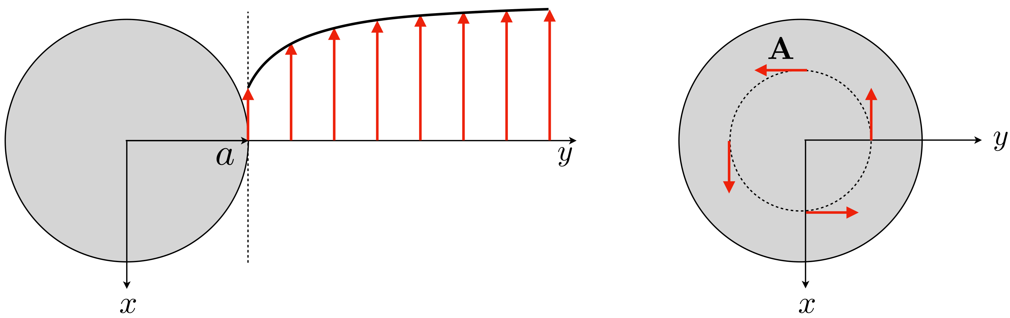
Let us check the functional form of the vector potential (Fig. 8.2).

(8.41)\[ \mathbf{A} = g(r) \mathbf{e}_{r} \times \mathbf{u} = \frac{df}{dr} \mathbf{e}_{r} \times \mathbf{u} = \left( \frac{3a}{4} - \frac{a^{3}}{4r^{2}} \right) \mathbf{e}_{r} \times \mathbf{u}\]

Fig. 8.2 Vector potential: \(\mathbf{A}\) on the \(y\) axis (left); \(\mathbf{A}\) along a circle on a horizontal plane of \(z > 0\) (right).

For \(r \rightarrow \infty\),

(8.42)\[ \mathbf{A} \rightarrow \frac{3a}{4} \mathbf{e}_{r} \times \mathbf{u}\]

At \(r = a\),

(8.43)\[ \mathbf{A} = \frac{a}{2} \mathbf{e}_{r} \times \mathbf{u}\]

Therefore, \(|\mathbf{A}|\) increases as \(r\) increases. The spherical coordinates are taken to have the following base vectors:

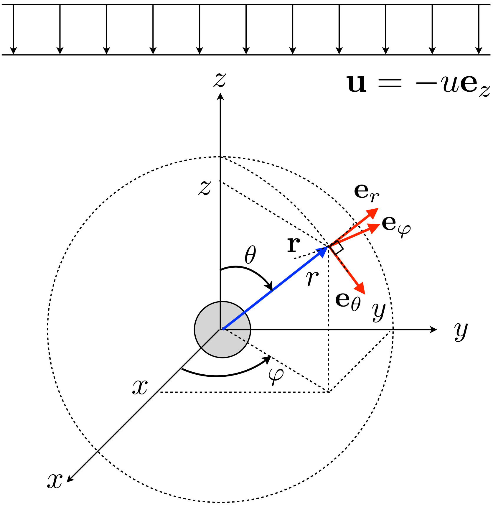
(8.44)\[\begin{split}\begin{split} &\mathbf{e}_{r} = \sin \theta \cos \varphi \mathbf{e}_{x}+\sin \theta \sin \varphi \mathbf{e}_{y}+\cos \theta \mathbf{e}_{z} \\ &\mathbf{e}_{\theta} = \cos \theta \cos \varphi \mathbf{e}_{x} + \cos \theta \sin \varphi \mathbf{e}_{y} - \sin \theta \mathbf{e}_{z} \\ &\mathbf{e}_{\varphi} = - \sin \varphi \mathbf{e}_{x} + \cos \varphi \mathbf{e}_{y} \end{split}\end{split}\]

and the uniform velocity \(\mathbf{u}\) directs toward \(-z\), where \(\theta\) is the polar coordinate and \(\varphi\) is the azimuthal coordinate. Note that this definition is different from that used in Landau and Lifshitz. On the \(y\) axis (\(\theta = \pi/2\)), \(\mathbf{e}_{r} \times \mathbf{u} = - u \mathbf{e}_{x}\) and \(|\mathbf{A}|\) increases with increasing \(y\), so that \(\nabla \times \mathbf{A}\) produces vectors with direction opposite to \(\mathbf{u}\). Especially, at \(r = a\), \(\nabla \times \mathbf{A} = - \mathbf{u}\) and \(\mathbf{v} = 0\). Around the \(z\) axis (\(\theta \sim 0\)), \(\mathbf{e}_{r} \times \mathbf{u}\) gives vectors along the \(\varphi\) coordinate line. The vector field \(\mathbf{e}_{r} \times \mathbf{u}\) along the coordinate line looks rotating in the \(+\varphi\) direction, so that, roughly speaking, \(\nabla \times \mathbf{A}\) gives vectors directing toward \(+z\) so as to retard the flow around the sphere.

The pressure field can be obtained from Eq. (8.3):

(8.45)\[ \nabla p = \mu \nabla^{2} \mathbf{v} \]

By substituting Eq. (8.14), we have

(8.46)\[ \nabla p = \mu \nabla^{2} ( \nabla \times \nabla \times ( f \mathbf{u} ) + \mathbf{u} ) = \mu \nabla^{2} \nabla \times \nabla \times ( f \mathbf{u} )\]

where \(\nabla^{2} \mathbf{u} = 0\) was used. Using the identity \(\nabla \times \nabla \times (\text{any vector}) = \nabla (\nabla \cdot (\text{any vector})) - \nabla^{2} (\text{any vector})\) and making some interchange in the order of the differential operators yields

(8.47)\[ \nabla p = \nabla \mu \nabla^{2} \nabla \cdot f \mathbf{u} - \mu \mathbf{u} \nabla^{2} \nabla^{2} f\]

However, due to Eq. (8.24),

(8.48)\[ \nabla p = \nabla \mu \nabla^{2} \nabla \cdot f \mathbf{u} \]

Integrating this equation yields

(8.49)\[ p = \mu \nabla^{2} \nabla \cdot f \mathbf{u} + p_{0}\]

where \(p_{0}\) is the far field pressure. The first term on the R.H.S. can be rewritten as

(8.50)\[ \mu \nabla^{2} \nabla \cdot f \mathbf{u} \rightarrow \mu \frac{\partial^{2}}{\partial x_{k} \partial x_{k}} \frac{\partial f u_{j}}{\partial x_{j}} = \mu u_{j} \frac{\partial }{\partial x_{j}} \frac{\partial^{2} f}{\partial x_{k} \partial x_{k}} \rightarrow \mu \mathbf{u} \cdot \nabla ( \nabla^{2} f )\]

Again we use Eq. (8.26) for the Laplacian of \(f\) and we obtain

(8.51)\[ p = 2 \alpha \mu \mathbf{u} \cdot \nabla \frac{1}{r}+ p_{0}\]

Using \(\nabla r^{n} = n r^{n-1} \mathbf{e}_{r}\) and \(\alpha = 3a/4\), we have

(8.52)\[ p = p_{0} - \frac{3 \mu a ( \mathbf{u} \cdot \mathbf{e}_{r} )}{2 r^{2}}\]

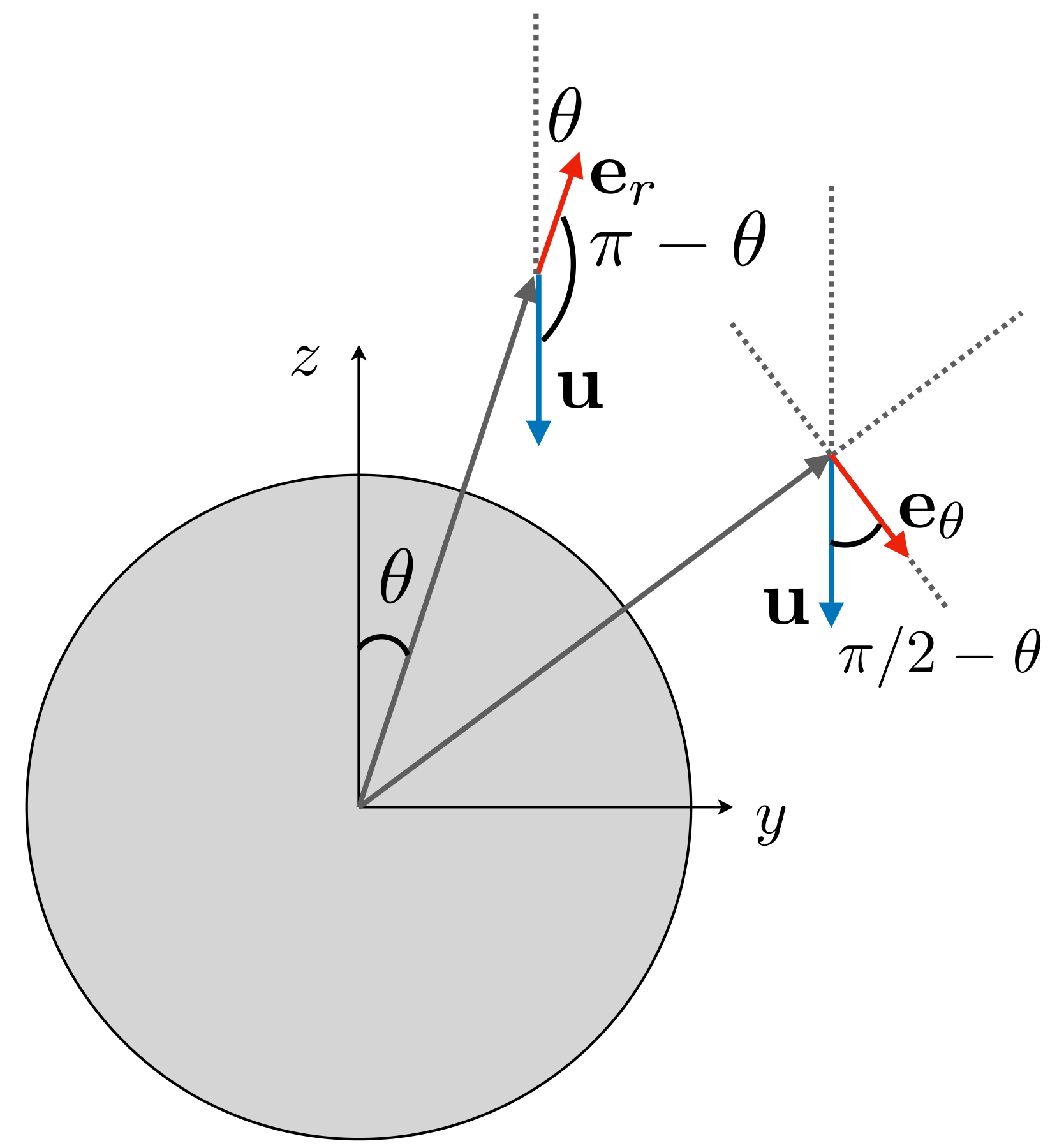
The drag force acting of the sphere is calculated in the following. The velocity components are (refer Fig. 8.3 for the calculation of the dot products between the velocity and the base vectors.)

(8.53)\[\begin{split}\begin{split} &v_{r} = \mathbf{v} \cdot \mathbf{e}_{r} = \mathbf{u} \cdot \mathbf{e}_{r} \left( 1 - \frac{3a}{2r} + \frac{a^{3}}{2 r^{3}} \right) = - u \cos \theta \left( 1 - \frac{3a}{2r} + \frac{a^{3}}{2 r^{3}} \right) \\ &v_{\theta} = \mathbf{v} \cdot \mathbf{e}_{\theta} = \mathbf{u} \cdot \mathbf{e}_{\theta} \left( 1 - \frac{3a}{4r} - \frac{a^{3}}{4 r^{3}} \right) = u \sin \theta \left( 1 - \frac{3a}{4r} - \frac{a^{3}}{4 r^{3}} \right) \end{split}\end{split}\]

(8.54)\[ p = p_{0} + \frac{3 \mu a u}{2 r^{2}} \cos \theta\]

Fig. 8.3 Direction cosine for the base vectors and the unit vector \(\mathbf{u}/u\).}

Some components of the viscous stress tensor are

(8.55)\[ \tau_{rr} = 2 \mu \frac{\partial v_{r}}{\partial r} = - 2 \mu u \cos \theta \left( \frac{3 a}{2 r^{2}} - \frac{3 a^{3}}{2 r^{4}} \right)\]

(8.56)\[ \tau_{r\theta} = \mu \left( \frac{1}{r} \frac{\partial v_{r}}{\partial \theta} + \frac{\partial v_{\theta}}{\partial r} - \frac{v_{\theta}}{r} \right) = \frac{3 \mu u a^{3}}{2 r^{4}} \sin \theta\]

At \(r = a\),

(8.57)\[ \left. p \right|_{r=a} = p_{0} + \frac{3 \mu u}{2 a} \cos \theta\]

(8.58)\[ \left. \tau_{rr} \right|_{r=a} = 0\]

(8.59)\[ \left. \tau_{r\theta} \right|_{r=a} = \frac{3 \mu u}{2 a} \sin \theta\]

The force acting on the sphere is given by

(8.60)\[ \mathbf{F} = \iint_{S} (-p \mathbf{I} + \boldsymbol{\tau}) \cdot \mathbf{n} dS\]

where \(\mathbf{n} = \mathbf{e}_{r}\). The drag \(F_{D}\) is the component of \(\mathbf{F}\) in the \(-z\) direction; hence

(8.61)\[ F_{D} = -\mathbf{e}_{z} \cdot \mathbf{F} = \iint_{S} (p \mathbf{e}_{z} \cdot \mathbf{I} \cdot \mathbf{e}_{r} -\mathbf{e}_{z} \cdot \boldsymbol{\tau} \cdot \mathbf{e}_{r}) dS = \iint_{S} (p \mathbf{e}_{z} \cdot \mathbf{e}_{r} - \mathbf{e}_{z} \cdot \boldsymbol{\tau} \cdot \mathbf{e}_{r}) dS\]

For the pressure term, \(\mathbf{e}_{z} \cdot \mathbf{e}_{r} = \cos \theta\). By expanding the viscous stress, we obtain

(8.62)\[\begin{split}\begin{split} \mathbf{e}_{z} \cdot \boldsymbol{\tau} \cdot \mathbf{e}_{r} &= \mathbf{e}_{z} \cdot ( \tau_{rr} \mathbf{e}_{r} \mathbf{e}_{r} + \tau_{r\theta} \mathbf{e}_{r} \mathbf{e}_{\theta} + \tau_{r\varphi} \mathbf{e}_{r} \mathbf{e}_{\varphi} + \tau_{\theta r} \mathbf{e}_{\theta} \mathbf{e}_{r} + \tau_{\theta \theta} \mathbf{e}_{\theta} \mathbf{e}_{\theta} + \tau_{\theta \varphi} \mathbf{e}_{\theta} \mathbf{e}_{\varphi} + \tau_{\varphi r} \mathbf{e}_{\varphi} \mathbf{e}_{r} + \tau_{\varphi \theta} \mathbf{e}_{\varphi} \mathbf{e}_{\theta} + \tau_{\varphi \varphi} \mathbf{e}_{\varphi} \mathbf{e}_{\varphi} ) \cdot \mathbf{e}_{r} \\ &= \mathbf{e}_{z} \cdot ( \tau_{rr} \mathbf{e}_{r} + \tau_{\theta r} \mathbf{e}_{\theta} + \tau_{\varphi r} \mathbf{e}_{\varphi} ) = \tau_{rr} \mathbf{e}_{z} \cdot \mathbf{e}_{r} + \tau_{\theta r} \mathbf{e}_{z} \cdot \mathbf{e}_{\theta} \\ &= \tau_{rr} \cos \theta - \tau_{\theta r} \sin \theta \end{split}\end{split}\]

where \(\tau_{\varphi r} = 0\) because of the symmetry of the flow, and \(\mathbf{e}_{z} \cdot \mathbf{e}_{r} = \cos \theta\) and \(\mathbf{e}_{z} \cdot \mathbf{e}_{\theta} = -\sin \theta\) were used. Putting this result into the integration yields

(8.63)\[ F_{D} = \iint_{S} (p \cos \theta - \tau_{rr} \cos \theta + \tau_{\theta r} \sin \theta) dS\]

Substituting Eqs. (8.57), (8.58) and (8.59) into this equation gives

(8.64)\[ F_{D} = \int_{0}^{2 \pi} \int_{0}^{\pi} \left( p_{0} \cos \theta + \frac{3 \mu u}{2 a} \cos^{2} \theta + \frac{3 \mu u}{2 a} \sin^{2} \theta \right) a^{2} \sin \theta d \theta d \varphi \]

It should be noted that the surface integral of any constant vanishes. Hence \(p_{0}\) has no contribution to the results.

(8.65)\[\begin{split}\begin{split} F_{D} &= \int_{0}^{2 \pi} \int_{0}^{\pi} \left( \frac{3 \mu u}{2 a} \cos^{2} \theta + \frac{3 \mu u}{2 a} \sin^{2} \theta \right) a^{2} \sin \theta d \theta d \varphi = 3 \pi \mu u a \int_{0}^{\pi} \sin \theta d \theta \\ &= 6 \pi \mu u a \end{split}\end{split}\]

The drag coefficient defined by

(8.66)\[ C_{D} = \frac{F_{D}}{\frac{1}{2} \rho u^{2} \pi a^{2}}\]

is then obtained as

(8.67)\[ C_{D} = \frac{24}{Re}\]

where \(Re\) is the Reynolds number defined by

(8.68)\[ Re = \frac{2 \rho u a}{\mu}\]