2.1. Averaged quantities

References

• Zuber and Findlay [ZF65]: Drift-flux model

Flow structures in two-phase flows show a significant variety. At a relatively small gas volume flux, the gas phase injected into a vertical pipe filled with still liquid may form rising bubbles. Bubble flows are termed bubbly flows. With increasing gas flow rate, two-phase co-current flows in a vertical pipe may include large bubbles in a bullet-like shape followed by small bubbles in liquid slug. This flow structure is called a slug flow. A very high gas flow rate allows the gas phase to form a gas core in the center region of a pipe, and the liquid phase pushed out toward the pipe wall takes a ring-like shape; therefore, this flow pattern is referred to as annular flow. In between the slug and annular flows, we may observe a more complicated flow characteristics; referred to as a churn flow. Fig. 2.1 shows a flow pattern map drawn by using Mishima-Ishii’s criteria [MI84].

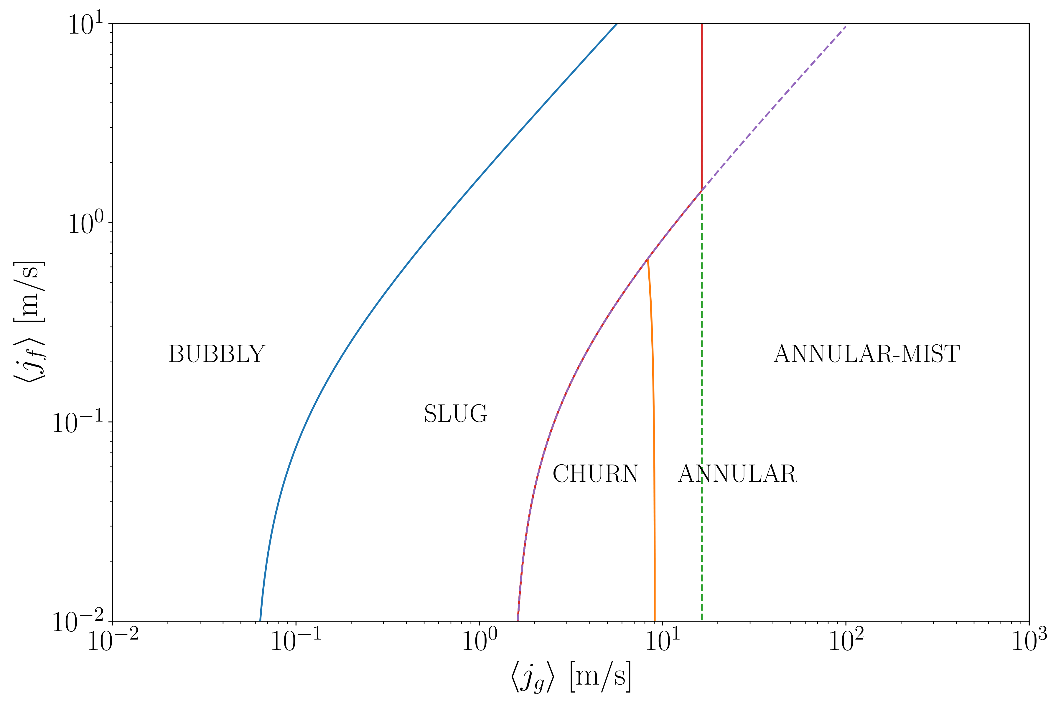
Fig. 2.1 Flow pattern map drawn by Mishima-Ishii criteria for air-water system in 20 mm pipe. The horizontal and vertical axes are the gas and liquid volumetric fluxes.

It is of course very difficult to understand everything about complex two-phase dynamics; however, for engineering purposes, simplified models are of great use for the design of industrial devices. We discuss the drift-flux model, which is a general approach to estimate the volume fraction of the two phases only with two model parameters.

Estimating the volume fraction of each phase in the two-phase system is important in the design and operation of two-phase flow devices. The drift-flux model [ZF65] is one of the simplified approaches for the estimation of the volume fraction. The simple principle realizes wide-range applicability, and the model has been utilized in many applications. The drift-flux model uses averaging to extract only two model parameters that represent the two-phase flow characteristics, that is, the distribution parameter \(C_{0}\) and the drift velocity \(v_{kj}\). A brief description of the model derivation is given in the following.

The phase indicator defined by the following equation is a numerical tool to represent the state of the position \(\mathbf{x}\) at time \(t\); which phase occupies that space:

(2.1)\[\begin{split} X_{k} (\mathbf{x}, t) = \left\{ \begin{array}{ll} 1 &\text{if}~~\mathbf{x} \in \text{phase}~k \\ 0 &\text{otherwise} \end{array} \right.\end{split}\]

The local volume fraction is defined by

(2.2)\[ \alpha_{k} (\mathbf{x}, t) = \frac{1}{T} \int_{t - T/2}^{t + T/2} X_{k} (\mathbf{x}, t) dt\]

The time duration \(T\) may be taken as small as possible such that \(\alpha_{k}\) is an instantaneous quantity, but should be set finite to make \(\alpha_{k}\) statistically meaningful. For the gas phase \(k = G\), \(\alpha_{G}\) is called the void fraction. See Fig. 2.2 for a schematic description of the definitions.

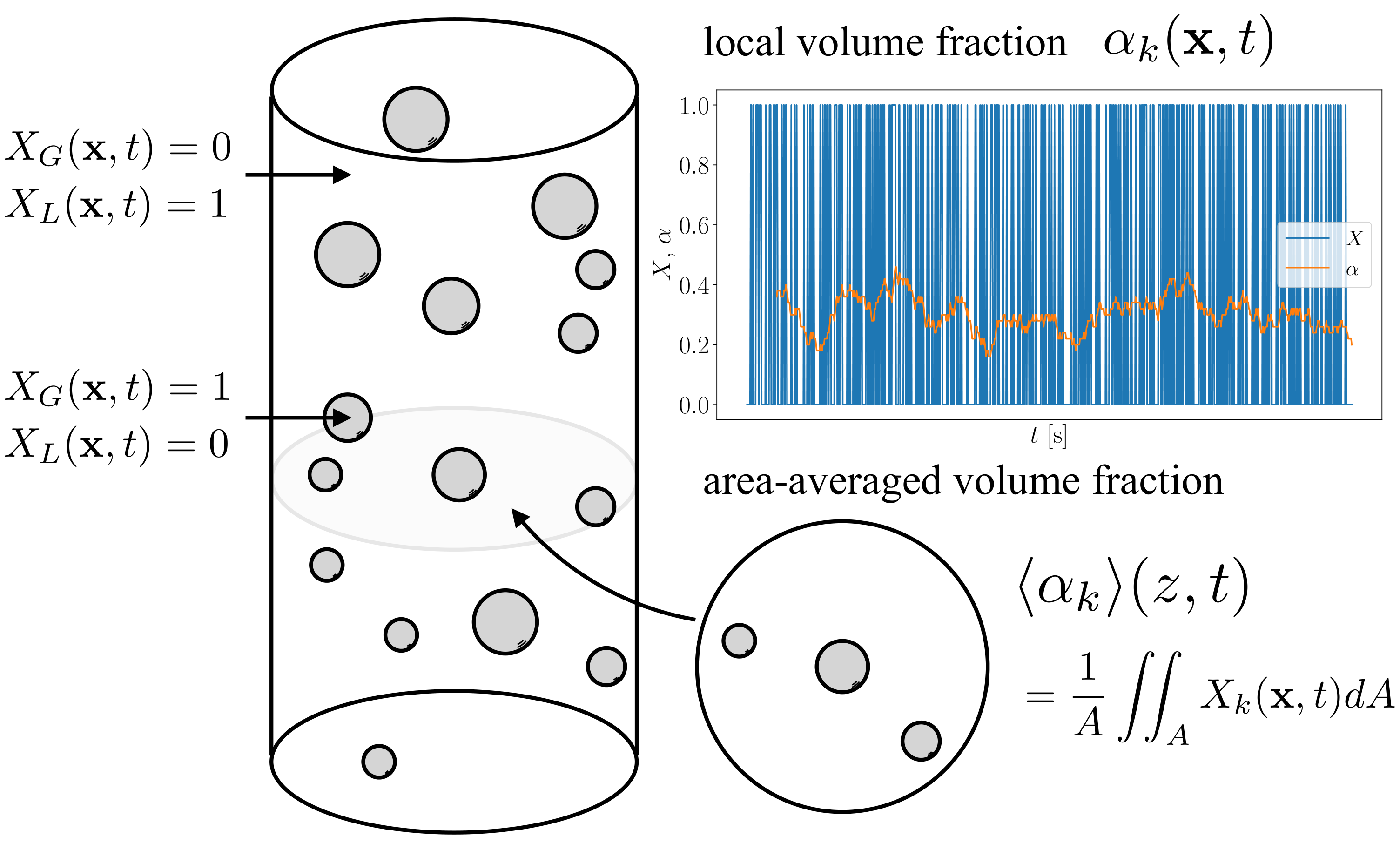
Fig. 2.2 Volume fraction

The velocity field of the two-phase flow is described by the local instantaneous velocity: \(\mathbf{v} (\mathbf{x}, t)\). The local volumetric flux is defined as the \(X\)-weighted time-average of the fluid velocity:

(2.3)\[ \mathbf{j}_{k} (\mathbf{x}, t) = \frac{1}{T} \int_{t-T/2}^{t+T/2} X_{k} \mathbf{v} dt\]

This operation extracts the local instantaneous velocity of the \(k\)th phase. The total volumetric flux is defined as the sum of the fluxes of each phase:

(2.4)\[ \mathbf{j} = \sum_{k=1,2} \mathbf{j}_{k}\]

The phase-averaged (local) quantities are generally written as

(2.5)\[ f_{k} (\mathbf{x}, t) = \frac{\frac{1}{T} \int X_{k} f dt}{\frac{1}{T} \int X_{k} dt} = \frac{\frac{1}{T} \int X_{k} fdt}{\alpha_{k}}\]

Taking \(f = \mathbf{v}\) yields the phase-averaged velocity:

(2.6)\[ \mathbf{v}_{k} (\mathbf{x}, t) = \frac{\frac{1}{T} \int_{t-T/2}^{t+T/2} X_{k} \mathbf{v} dt}{\frac{1}{T} \int_{t-T/2}^{t+T/2} X_{k} dt} = \frac{\mathbf{j}_{k}}{\alpha_{k}}\]

Therefore,

(2.7)\[ \mathbf{j}_{k} = \alpha_{k} \mathbf{v}_{k}\]

The local relative velocity between the two phases is defined by

(2.8)\[ \mathbf{v}_{R} = \mathbf{v}_{2} - \mathbf{v}_{1}\]

An alternative representation of the velocity difference is the local drift velocity defined by

(2.9)\[ \mathbf{v}_{kj} = \mathbf{v}_{k} - \mathbf{j}\]

If we assume that the two fluids form a homogeneous two-phase mixture, there is no relative motion between the two phases, i.e. \(\mathbf{v}_{R} = 0\), and therefore \(\mathbf{v}_{k} = \mathbf{j}\) and \(\mathbf{v}_{kj} = 0\), corresponding to the homogeneous model.