11.3. Bretherton problem

Summary

• Subject: Large bubble in small conduits

• Main conclusion: Scaling of liquid film thickness: \(\delta/R \propto Ca^{2/3}\)

• Key idea Small scale of conduit facilitates analysing bubble shape as lubrication problem.

• References:

  • Bretherton [Bre61]

  • Magnini et al. [MKM+19]

  • de Ryck [dR02]

Magnini et al. [MKM+19] analyzed the motion of a Taylor bubble rising through a vertical circular pipe. They introduced the following dimensionless variables:

(11.41)\[ \hat{u} = \frac{u}{U}, \quad \hat{v} = \frac{v}{V}, \quad \hat{x} = \frac{x}{\ell}, \quad \hat{y} = \frac{y}{h_{0}}, \quad \hat{p} = \frac{p}{\mu U \ell / h_{0}^{2}}, \quad \hat{h} = \frac{h}{h_{0}}, \quad \hat{\kappa} = \frac{\kappa}{h_{0} / \ell^{2}}\]

where \(u\) and \(v\) are the axial and radial velocity components, \(p\) is the pressure, \(h\) is the thickness of the liquid film formed between the bubble surface and the pipe wall, \(\kappa\) is the curvature of the bubble surface, \(\rho\) is the liquid density, \(\mu\) is the liquid viscosity, and they are nondimensionalized by the characteristic velocity \(U = U_{b}\) in the axial direction, \(V = h_{0} U_{b}/\ell\) in the radial direction, the liquid film thickness \(h_{0}\) in the fully developed film region, and the characteristic length of the dynamic meniscus \(\ell\), where \(\epsilon = h_{0} / \ell \ll 1\). We use the frame of reference moving with the bubble; therefore, in the steady state, we have

(11.42)\[ \hat{u}_{x} + \hat{v}_{y} = 0\]

(11.43)\[ \frac{1}{2} Ca_{b}^{1/3} Re_{b} H \left( \hat{u} \hat{u}_{\hat{x}} + \hat{v} \hat{u}_{\hat{y}} \right) = -\hat{p}_{\hat{x}} + \hat{u}_{\hat{y}\hat{y}} - T^{2}\]

(11.44)\[ \hat{p}_{\hat{y}} = 0\]

where the orders, \(H = O(\epsilon^{2})\), \(Ca_{b} = O(\epsilon^{3})\) and \(Bo = O(\epsilon^{-1})\), were used, and

(11.45)\[ H = \frac{h_0}{R}, \quad Ca_b = \frac{\mu U_b}{\sigma}, \quad Re_b = \frac{2 \rho U_b R}{\mu}, \quad Bo = \frac{\rho g R^2}{\sigma}, \quad T^{2} = H^{2} \frac{Bo}{Ca_{b}}\]

where \(\sigma\) is the surface tension, and \(R\) is the pipe radius. The boundary conditions are

(11.46)\[ \hat{u}_{\hat{y}} = 0~~~~\text{and}~~~~\hat{p} = - \hat{\kappa}~~~~\text{at}~~\hat{y} = \hat{h}(\hat{x})\]

(11.47)\[ \hat{u} = -1~~~~\text{and}~~~~\hat{v} = 0~~~~\text{at}~~\hat{y} = 0\]

In the following, we omit hat for simplicity.

The following parabolic velocity profile is assumed for the dynamic meniscus region:

(11.48)\[ u(x, y) = 3 F(x) \left( \frac{y^{2}}{2} - h y \right) - 1\]

It should be noted that \(h\) is a function of \(x\). This function satisfies the boundary condition \(u = 0\) at \(y = 0\). The volume flow rate passing through the dynamic meniscus regions is therefore

(11.49)\[ Q = \int_{0}^{h} u(x,y) dy = - F(x) h^{3} - h\]

The momentum equation is given by

(11.50)\[ \frac{1}{2} \text{Ca}_{b}^{1/3} \text{Re}_{b} H(uu_{x} + vu_{y}) = - p_{x} + u_{yy} - T^{2}\]

However, in the fully-developed film, \(u_{x} = v = 0\), so that

(11.51)\[ 0 = - p_{x} + u_{yy} - T^{2}\]

Therefore, the velocity equation in the developed film is the same as that for the case of negligible inertia:

(11.52)\[ u_{CD}(y) = T^{2} \left( \frac{y^{2}}{2} - y \right) - 1\]

The shear free condition is satisfied, i.e., \(du_{CD}/dy = 0\) at \(y = 1\). When \(T = 0\), \(u_{CD}=-1\), which means that the film is stagnant. The dimensionless film thickness is \(h = 1\) in the developed film; therefore, the flow rate is given by

(11.53)\[ Q = \int_{0}^{1} u_{CD} dy = - \frac{T^{2}}{3} - 1\]

Equating the expressions of the flow rate gives the function \(F\), that is,

(11.54)\[ F(x) = \frac{1}{h^{3}} \left( \frac{T^{2}}{3} + 1 - h \right)\]

Then,

(11.55)\[ u(x, y) = \frac{3}{h^{3}} \left( \frac{T^{2}}{3} + 1 - h \right) \left( \frac{y^{2}}{2} - h y \right) - 1\]

We integrate the momentum equation to obtain the curvature equation:

(11.56)\[ \frac{1}{2} \text{Ca}_{b}^{1/3} \text{Re}_{b} H \left[ \int_{0}^{h} u u_{x} dy + \int_{0}^{h} v u_{y} dy \right] = \int_{0}^{h} \kappa_{x} dy + \int_{0}^{h} u_{yy} dy - \int_{0}^{h} T^{2} dy\]

The second derivative of \(u\) with respect to \(y\) is

(11.57)\[ u_{yy} = \frac{3(1 - h) + T^{2}}{h^{3}}\]

The integration of the right hand side gives

(11.58)\[ \int_{0}^{h} \kappa_{x} dy + \int_{0}^{h} u_{yy} dy - \int_{0}^{h} T^{2} dy = h \left\{ \kappa_{x} + T^{2} \frac{1 - h^{3}}{h^{3}} + 3 \frac{1 - h}{h^{3}} \right\}\]

which is of course the same as observed in the negligible inertia case. We need the expressions of the first derivatives of \(u\) and \(v\) to integrate the left hand side. The first derivatives are

(11.59)\[ u_{x} = \frac{ \left(6 h - 3 T^{2} - 9 \right) h_{x} y^2 + \left( \left( 4 T^{2} + 12 \right) h - 6 h^2 \right) h_{x} y} {2 h^{4}}\]

(11.60)\[ u_{y} = - \frac{\left(3 h - T^{2} - 3 \right) y - 3 h^{2} + \left( T^{2} + 3 \right) h}{h^{3}}\]

From the continuity equation

(11.61)\[ u_{x} + v_{y} = 0\]

The radial velocity component can be obtained as

(11.62)\[ v = - \int_{0}^{y} u_{x} (x, \eta) d\eta\]

where \(v(0) = 0\) is used. Hence,

(11.63)\[ v(x, y) = - \frac{\left(2 h - T^{2} - 3 \right) h_{x} y^{3} + \left( \left( 2 T^{2} + 6 \right) h - 3 h^{2} \right) h_{x} y^2}{2 h^{4}}\]

By substituting these into the momentum equation and integrating the resultant equation, we obtain

(11.64)\[\begin{split} \int_{0}^{h} u u_{x} dy + \int_{0}^{h} v u_{y} dy = \frac{h_{x}}{5 h^{2}} \left(h^{2} - 6 - 4T^{2} - \frac{2}{3} T^{4} \right) \end{split}\]

Thus, the integrated momentum equation becomes

(11.65)\[ \text{Ca}_{b}^{1/3} \text{Re}_{b} H \frac{h_{x}}{10 h^{2}} \left(h^{2} - 6 - 4T^{2} - \frac{2}{3} T^{4} \right) = h \left\{ \kappa_{x} + \frac{3 ( 1 - h ) + T^{2}}{h^{3}} - T^{2} \right\}\]

Solving this equation for the curvature, we finally have

(11.66)\[ \kappa_{x} =3 \frac{h - 1}{h^{3}} + T^{2} \frac{h^{3} - 1}{h^{3}} + \frac{1}{10} H \text{Ca}_{b}^{1/3} \text{Re}_{b} \left(h^{2} - 6 - 4T^{2} - \frac{2}{3} T^{4} \right) \frac{h_{x}}{h^{3}}\]

A derivation of curvature equation up to \(\epsilon^{2}\) is also possible and was given by de Ryck [dR02] for the case in the absence of buoyancy. Fig. 11.4 shows a bubble shape computed using the de Ryck model. Some predictions of \(h\) at \(Re_{b}\) are shown in Fig. 11.5.

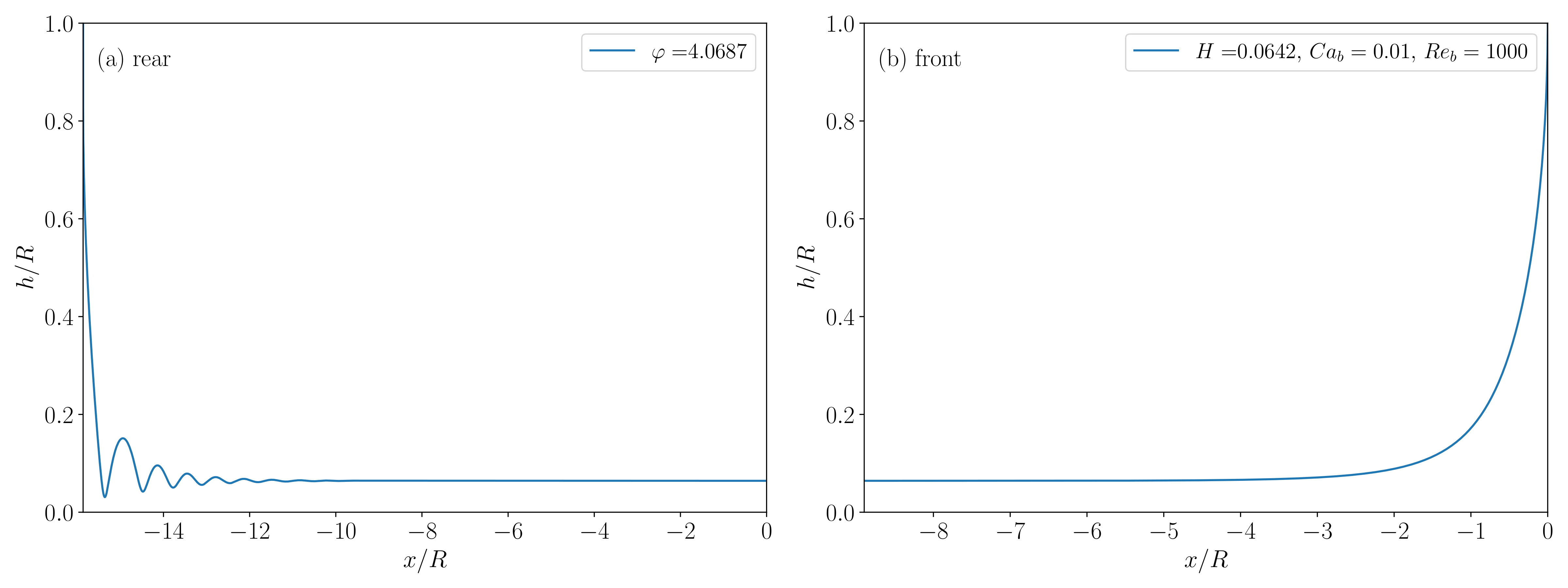
Fig. 11.4 The front and rear shapes for \(H = 0.642\), \(Ca_{b} = 0.01\) and \(Re_{b} = 1000\).

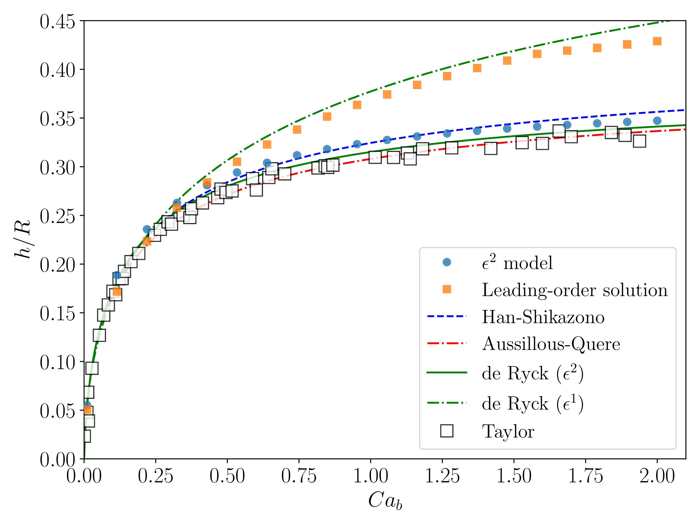
Fig. 11.5 Liquid film thickness \(h\) predicted by using the \(\epsilon^{2}\) model for \(Re_{b} = 0\). The \(\epsilon^{1}\) model [MKM+19] is substantially \(\epsilon^{0}\) since \(Re_{b} = 0\). The predictions are compared with the de Ryck’s result and the Han-Shikazono correlation. The curved for de Ryck’s predictions are fitting in the form of \(h/R = a Ca_{b}^{c}/(1 + b Ca_{b}^{c})\) for data points quoted from the figures in de Ryck [dR02].