Water wave of infinitesimal amplitude

Referred from

Wave analogy for bubble rise velocity

As the basis of the wave analogy, let us briefly review the theory of water wave. Suppose that the water motion is irrotational and the flow is incompressible and two-dimensional. Let \(x\) be the horizontal axis along which water waves propagate. Let us have \(z\) as the vertical axis and the gravitational acceleration is given by \(\mathbf{g} = - g \mathbf{e}_{z}\). The water surface in equilibrium is \(z = 0\), while the displacement of surface from \(z = 0\) is denoted by \(\zeta (x, t)\) (see Fig. 6); therefore,

(146)\[ z = \zeta (x, t)\]

or

(147)\[ f (x, z, t) = z - \zeta (x, t) = 0\]

is the equation of surface. Since the flow is irrotational, there exists a velocity potential \(\phi\) produces \(\mathbf{v}\), i.e.,

(148)\[ \mathbf{v} = \nabla \phi\]

Substituting this equation into the continuity equation \(\nabla \cdot \mathbf{v} = 0\) yields

(149)\[ \nabla^{2} \phi = 0~~~~\text{or}~~~~\frac{\partial^{2} \phi}{\partial x^{2}} + \frac{\partial^{2} \phi}{\partial z^{2}} = 0\]

which is the Laplace equation holds in the water (\(- \infty < z < \zeta\)).

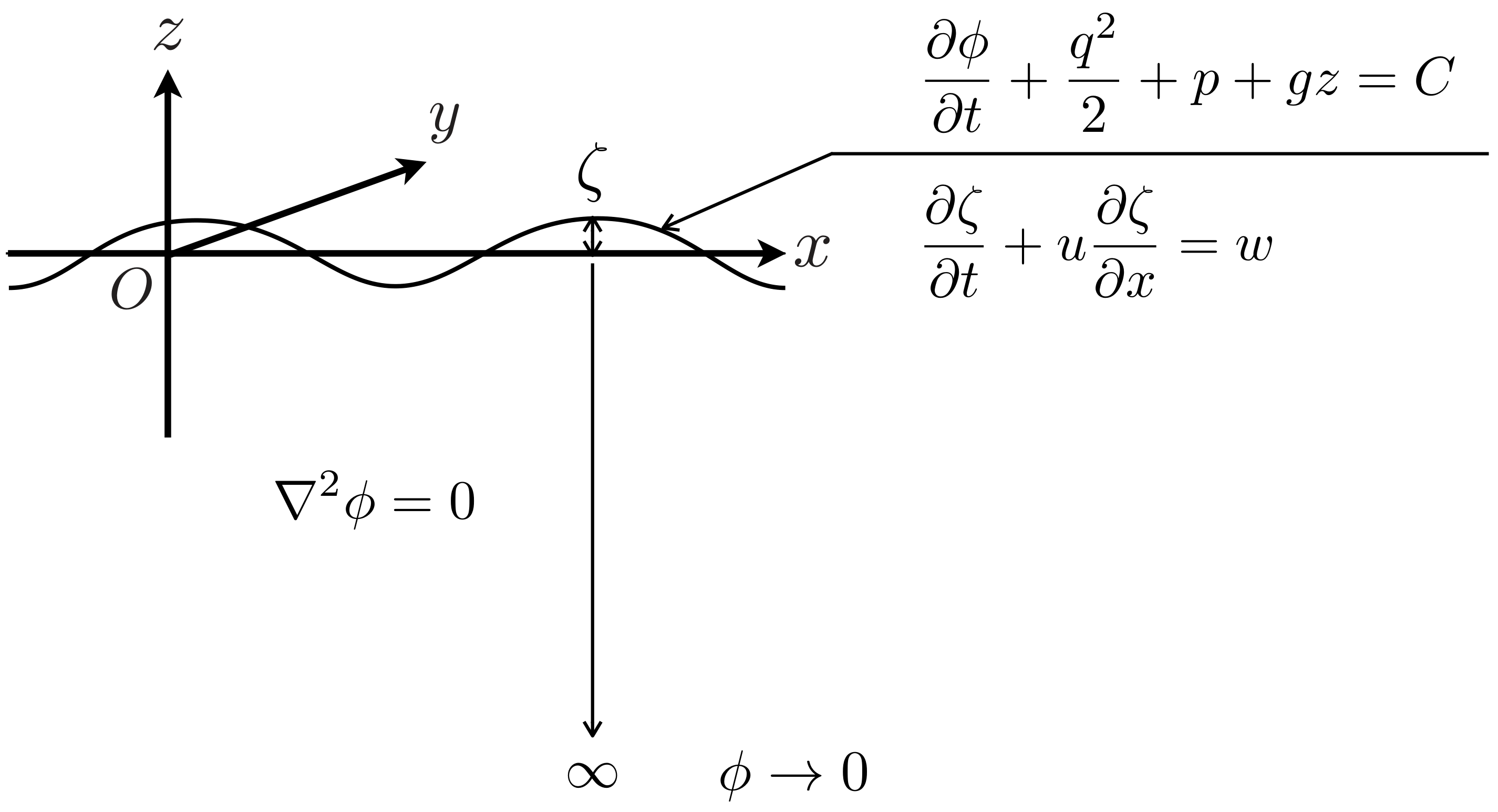
Fig. 6 Deep water wave

Fluid particles on the surface are always on the surface, in other words, the material derivative of \(f\) is zero:

(150)\[ \frac{Df}{Dt} = 0~~~~\text{or}~~~~\frac{\partial f}{\partial t} + u \frac{\partial f}{\partial x} + w \frac{\partial f}{\partial z} = 0~~~~\text{at}~~z = \zeta\]

where \(u\) and \(w\) are the velocity components in the \(x\) and \(z\) directions, respectively. By differentiating \(f\) in Eq. (147) we obtain \(\partial f / \partial t = - \partial \zeta / \partial t\), \(\partial f / \partial x = - \partial \zeta / \partial x\), and \(\partial f / \partial z = 1\). Using these relations, we have

(151)\[ \frac{\partial \zeta}{\partial t} + u \frac{\partial \zeta}{\partial x} = w~~~~\text{at}~~z = \zeta\]

This is the kinematic boundary condition at the water surface. The kinetic boundary condition is given by the following pressure equation:

(152)\[ \frac{\partial \phi}{\partial t} + \frac{q^{2}}{2} + \frac{p}{\rho} + gz = C\]

where \(q^{2} = \mathbf{v} \cdot \mathbf{v} = u^{2} + w^{2}\). The pressure at \(z = \zeta\) is \(p = p_{0} + \delta p\), where \(p_{0}\) is the atmospheric pressure, and \(\delta p\) is the pressure increase due to the action of surface tension.

(153)\[ \delta p = \sigma \kappa \]

where \(\kappa\) is the curvature of surface. The displacement \(\zeta\) can be regarded as the equation of a curve on the plane. The curvature of the curve is given by

A curve in the \(xy\) plane is given by a position vector \(\mathbf{r}(s)\), where \(s\) is the arc length of the curve and is used as the parameter. Differentiating \(\mathbf{r}\) with respect to \(s\) yields the unit tangential \(\mathbf{e}_{1} = d\mathbf{r}/ds = (dx/ds, dy/ds)\) to the curve. \(\mathbf{e}_{2} = (-dy/ds, dx/ds)\) is a unit vector right angle to \(\mathbf{e}_{1}\), so that \(\mathbf{e}_{1} \cdot \mathbf{e}_{2} = 0\). Differentiating this orthogonal condition, we have \(\dot{\mathbf{e}}_{1} \cdot \mathbf{e}_{2} + \mathbf{e}_{1} \cdot \dot{\mathbf{e}}_{2} = 0\), where dot denotes \(d/ds\). \(\dot{\mathbf{e}}_{1}\) gives a vector parallel to \(\mathbf{e}_{2}\). Therefore, we may write \(\dot{\mathbf{e}}_{1} = - \kappa \mathbf{e}_{2}\), where \(\kappa\) is the curvature of the curve. Substituting this into the above relationship gives \(\kappa = \mathbf{e}_{1} \cdot \dot{\mathbf{e}}_{2} = -(dx/ds)(d^{2}y/ds^{2}) + (dy/ds)(d^{2}x/ds^{2})\). However, the length of a line element on the curve is \(ds^{2} = dx^{2} + dy^{2} = (1 + d^{2}y/dx^{2}) dx^{2}\), and with this expression,

\[\begin{equation*} \kappa = \frac{- \partial^{2} y / \partial x^{2} }{\left[ 1 + \left( \partial y / \partial x \right)^{2} \right]^{3/2}} \end{equation*}\]

(154)\[ \kappa = \frac{- \frac{\partial^{2} \zeta}{\partial x^{2}}}{\left[ 1 + \left( \frac{\partial \zeta}{\partial x} \right)^{2} \right]^{3/2}}\]

where \(\kappa\) is positive when the water surface is convex to the water and is negative for concave shape. Taking \(C = p_{0} / \rho\), the boundary condition becomes

(155)\[ \frac{\partial \phi}{\partial t} + \frac{q^{2}}{2} + g\zeta + \frac{\sigma \kappa}{\rho} = 0~~~~\text{at}~~z = \zeta\]

In the following, we consider waves of infinitesimal amplitude. The velocity and the velocity potential of the water motion induced by the waves are also small, and therefore, the second and higher order perturbations are negligibly small. Therefore,

(156)\[ \frac{\partial \zeta}{\partial t} = \frac{\partial \phi}{\partial z}~~~~\text{at}~~z = 0\]

(157)\[ \frac{\partial \phi}{\partial t} + g \zeta - \frac{\sigma}{\rho} \frac{\partial^{2} \zeta}{\partial x^{2}} = 0~~~~\text{at}~~z = 0 \]

where we used the approximation \(\kappa \sim - \partial^{2} \zeta / \partial x^{2}\) for small \(\zeta\). Differentiating the second equation with respect to \(t\) gives

(158)\[ \frac{\partial^{2} \phi}{\partial t^{2}} + \left\{ g - \frac{\sigma}{\rho} \frac{\partial^{2} }{\partial x^{2}} \right\} \frac{\partial \zeta}{\partial t} = 0~~~~\text{at}~~z = 0 \]

and then combining this with the first equation yields the boundary condition expressed in terms of \(\phi\) only:

(159)\[ \frac{\partial^{2} \phi}{\partial t^{2}} + \left\{ g - \frac{\sigma}{\rho} \frac{\partial^{2} }{\partial x^{2}} \right\} \frac{\partial \phi}{\partial z} = 0~~~~\text{at}~~z = 0 \]

In addition to this integrated boundary condition at the surface, the boundary condition at the infinite depth is used to determine the solution of the Laplace equation:

(160)\[ q \rightarrow 0~~~~\text{as}~~z \rightarrow -\infty\]

Let us assume the solution in the form

(161)\[ \phi = f(z) \sin (kx - \omega t)\]

where \(k\) is the wave number and \(\omega\) is the angular frequency. Substituting this into the Laplace equation yields the following ODE of \(f(z)\):

(162)\[ \frac{d^{2}f}{dz^{2}} - k^{2} f = 0\]

Integrating this equation with the boundary condition at \(z \rightarrow -\infty\) yields

(163)\[ \phi = B e^{kz} \sin (kx - \omega t)\]

By substituting this into the boundary condition (159) we obtain the following dispersion relation:

(164)\[ \omega^{2} = \left( \frac{\sigma}{\rho} + \frac{g}{k^{2}} \right) k^{3}\]

By definition \(c_{p} = \omega / k\), we have

(165)\[ c_{p} = \sqrt{ \frac{2 \pi \sigma}{\rho \lambda} + \frac{g \lambda}{2 \pi} }\]

The phase velocity of water wave is shown in Fig. 7.

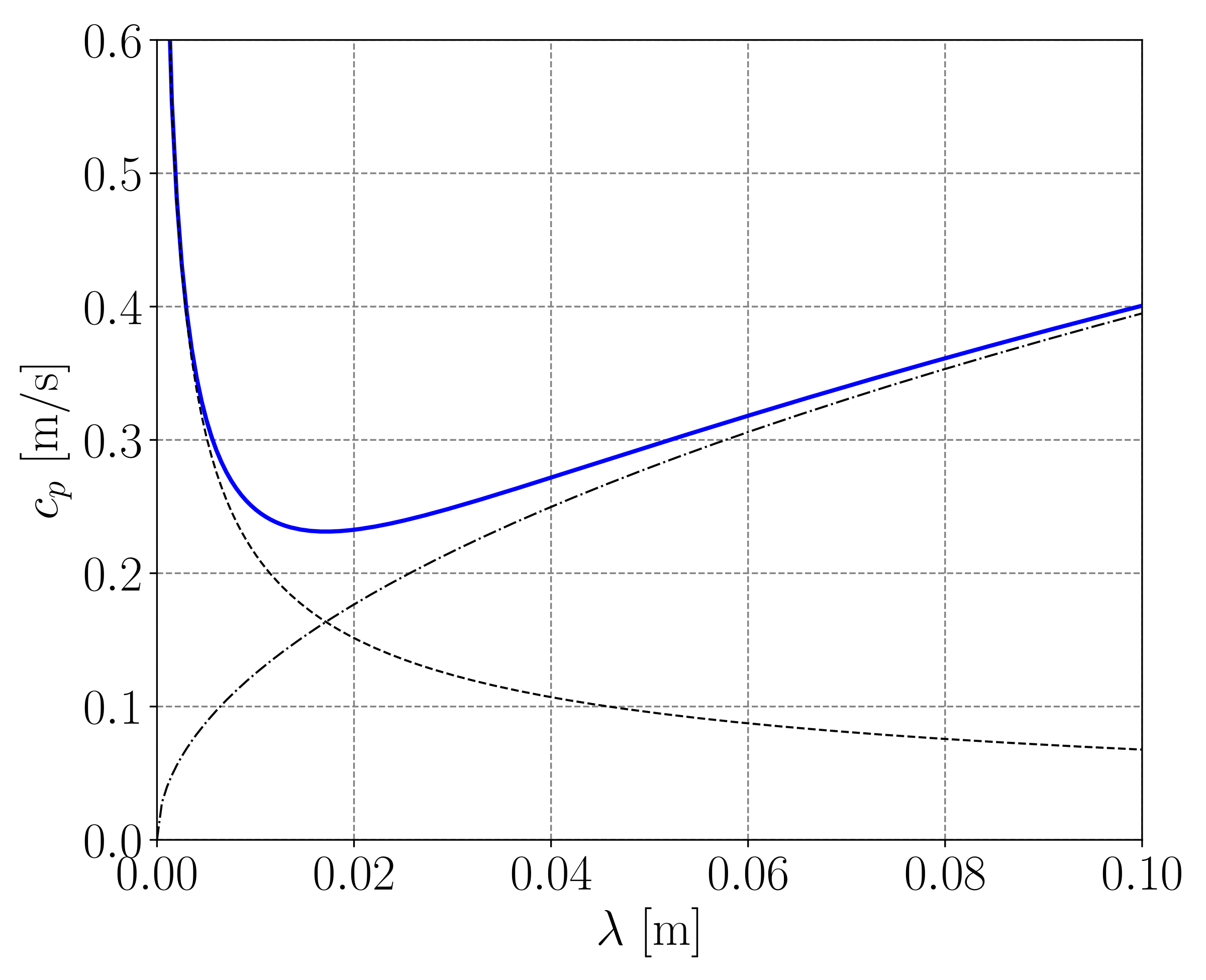
Fig. 7 Phase velocity of capillary-gravity wave