6.3. Shape deformation

Moore [Moo59] derived a bubble shape model for small perturbation from perfect sphere, that is the bubble shape is approximated as (Fig. 6.3)

(6.35)\[ r = a \left\{ 1 + \epsilon P_{2} (\cos \theta) \right\}\]

where \(r\) and \(\theta\) are the spherical coordinates, \(a\) is the radius of sphere, \(\epsilon~(\ll 1)\) is a small perturbation, and \(P_{2} (\cos \theta)\) is the second Legendre polynomial defined by

\(P_{0}(x) = 1\), \(P_{1}(x) = x\), \(P_{2}(x) = (3x^{2}-1)/2\), \(P_{3}(x) = (35x^{4}-30x^{2}+3)/8\) \(\cdots\).

The Legendre polynomials are orthogonal within \([-1, 1]\), that is \(\int_{-1}^{1} P_{m}(x) P_{n} dx = 2\delta_{mn}/(2n+1)\).

(6.36)\[ P_{2} (\cos \theta) = \frac{1}{2} \left( 3 \cos^{2} \theta - 1 \right)\]

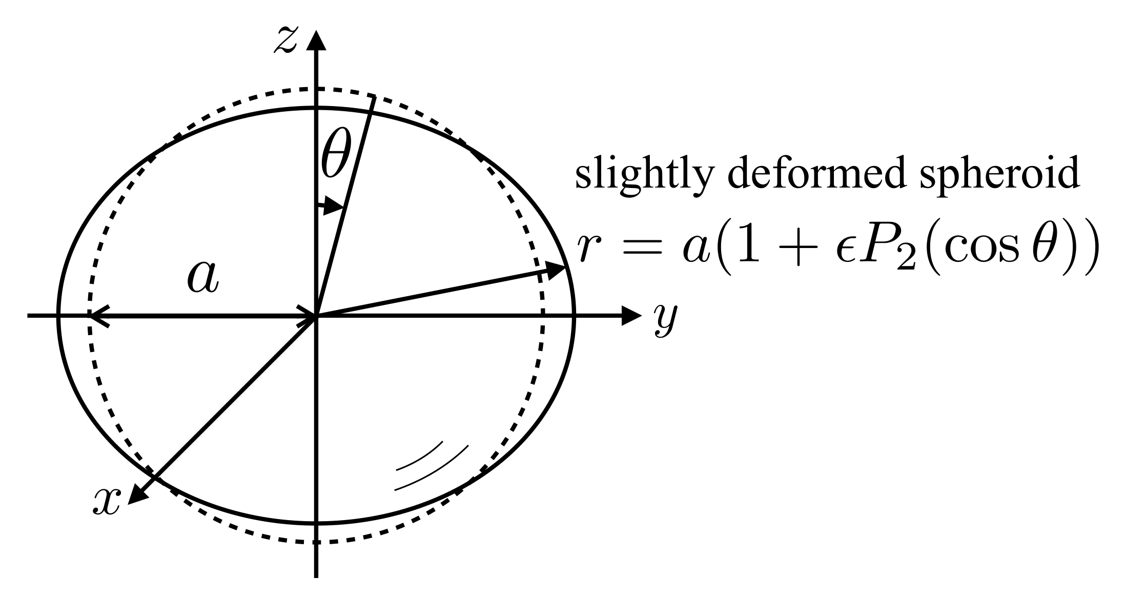
Fig. 6.3 Slightly deformed bubble

The tangential velocity components in a potential flow about a sphere moving a constant speed \(u\) is given by (Appendix Potential flow about sphere)

(6.37)\[ v_{\theta} = \frac{u a^{3}}{2 r^{3}} \sin \theta\]

Riding on the sphere, we observe

(6.38)\[ v_{\theta} = \frac{3 u a^{3}}{2 r^{3}} \sin \theta\]

Therefore,

(6.39)\[ p_{s} = p + \frac{1}{2} \rho q^{2} \sim p + \frac{1}{2} \rho v_{\theta}^{2}\]

(6.40)\[\begin{split}\begin{split} \frac{1}{2} \rho v_{\theta}^{2} &= \frac{1}{2} \rho \frac{9 u^{2} a^{6}}{4 r^{6}} \sin^{2} \theta \sim \frac{1}{2} \rho \frac{9 u^{2} a^{6}}{4 a^{6} (1 + \epsilon P_{2}(\cos \theta))^{6}} \sin^{2} \theta \sim \rho \frac{9 u^{2}}{8} (1 -6 \epsilon P_{2}(\cos \theta)) \sin^{2} \theta \\ &= \rho \frac{9 u^{2}}{8} \sin^{2} \theta + O(\epsilon \rho u^{2}) \end{split}\end{split}\]

At the stagnation point (\(\theta = 0\)),

(6.41)\[ p_{g} = p_{s} + \frac{2 \sigma}{a}\]

and for \(0 < \theta < \pi\),

(6.42)\[ p_{g} = p_{s} - \frac{1}{2} \rho u_{\theta}^{2} + \sigma \kappa\]

We need to calculate an approximate curvature \(\kappa\) at \(\theta\). The surface equation is given by

(6.43)\[ f = r - a (1 + \epsilon P_{2}(\cos \theta))\]

The normal to the isosurface of \(f\) is (see Appendix Continuity and NS equations in polar coordinate systems for differential operators)

(6.44)\[ \mathbf{N} = \left( \frac{\partial f}{\partial n}, \frac{1}{r} \frac{\partial f}{\partial \theta}, \frac{1}{r \sin \theta} \frac{\partial f}{\partial \varphi} \right) = \left( 1, \frac{3 a \epsilon}{r} \sin \theta \cos \theta, 0 \right)\]

The unit normal is therefore

(6.45)\[ \mathbf{n} = \frac{\mathbf{N}}{| \mathbf{N} |} = \frac{ \left( 1, \frac{3 a \epsilon}{r} \sin \theta \cos \theta, 0 \right) }{\left\{ {1 + \frac{9a^{2} \epsilon^{2}}{r^{2}} \sin^{2} \theta \cos^{2} \theta} \right\}^{1/2}}\]

However, for the first order,

(6.46)\[ \mathbf{n} = \left( 1, \frac{3 a \epsilon}{r} \sin \theta \cos \theta, 0 \right)\]

The curvature can be calculated as the divergence of the field of \(\mathbf{n}\), that is

(6.47)\[\begin{split}\begin{split} \kappa &= \nabla \cdot \mathbf{n} = \frac{1}{r^{2}} \frac{\partial r^{2} n_{r} }{\partial r} + \frac{1}{r \sin \theta} \frac{\partial n_{\theta} \sin \theta}{\partial \theta} + \frac{1}{r \sin \theta} \frac{\partial n_{\varphi}}{\partial \varphi} \\ &\sim \frac{2}{r} + \frac{3 a \epsilon}{2} \left(2 - 3 \sin^{2} \theta \right) = \frac{2}{r} + \frac{3 a \epsilon}{r^{2}} P_{2} (\cos \theta) \end{split}\end{split}\]

Substituting \(r = a (1 + \epsilon P_{2}(\cos \theta))\) yields

(6.48)\[ \kappa = \frac{2}{a} (1 - \epsilon P_{2}(\cos \theta)) + \frac{3 \epsilon}{a} (1 - 2 \epsilon P_{2}(\cos \theta)) P_{2} (\cos \theta) \sim \frac{2}{a} + \frac{4 \epsilon}{a} P_{2}(\cos \theta) + O \left( \frac{\epsilon^{2}}{a} \right)\]

Therefore,

(6.49)\[ p_{g} = p_{s} - \rho \frac{9 u^{2}}{8} \sin^{2} \theta - O(\epsilon \rho u^{2}) + \sigma \left\{ \frac{2}{a} \left( 1 + 2 \epsilon P_{2} (\cos \theta) \right) + O \left( \frac{\epsilon^{2}}{a} \right) \right\}\]

Subtracting Eq. (6.41) from Eq. (6.49) yields

(6.50)\[ \rho \frac{9 u^{2}}{8} \sin^{2} \theta + O(\epsilon \rho u^{2}) = \frac{4 \sigma \epsilon}{a} P_{2} (\cos \theta) + O \left( \frac{\sigma \epsilon^{2}}{a} \right)\]

The Legendre polynomial can be written as

(6.51)\[ P_{2} (\cos^{2} \theta) = \frac{1}{2} (\cos^{2} \theta - 1) = 1 - \frac{3}{2} \sin^{2} \theta \]

Hence,

(6.52)\[ \rho \frac{9 u^{2}}{8} \sin^{2} \theta + O(\epsilon \rho u^{2}) = \frac{4 \sigma \epsilon}{a} \left( 1 - \frac{3}{2} \sin^{2} \theta \right) + O \left( \frac{\sigma \epsilon^{2}}{a} \right)\]

Considering the balance between the terms depending on \(\sin^{2} \theta\), we find

(6.53)\[ \epsilon = - \frac{3}{16} \frac{\rho u^{2} a}{\sigma} \]

Using the definition of the Weber number, \(We = 2 \rho u^{2} a / \sigma\), we have

(6.54)\[ \epsilon = - \frac{3}{32} We\]

The definition of \(We\) used here can be considered as the same as that with the sphere-volume-equivalent bubble diameter since the perturbation from spherical shape is small enough. The coordinates of the surface at \(\theta = 0\) and \(\pi/2\) are

(6.55)\[ r = a (1 + \epsilon)~~(\theta = 0),~~~~r = a (1 - \epsilon/2)~~(\theta = \pi/2) \]

The aspect ratio (the major axis / the minor axis) of the bubble is therefore given by

(6.56)\[ \chi = \frac{a (1 - \epsilon / 2)}{a (1 + \epsilon)} \sim (1 - \epsilon/2)(1 - \epsilon) \sim 1 - \frac{3}{2} \epsilon = 1 + \frac{9}{64} We\]

The bubble shape is hence oblate spheroid and the deformation increases linearly as the Weber number increases.

Moore [Moo65] attempted to exactly satisfy the boundary conditions at the stagnation point and at the bubble equator, which resulted in

(6.57)\[ We = \frac{ 4 (\chi^3 + \chi - 2) [\chi^2 \sec^{-1} \chi - (\chi^2 - 1)^{\frac{1}{2}}]^2 }{\chi^{\frac{4}{3}} (\chi^2 - 1)^{3}}\]

The bubble shape models are compared in Fig. 6.4. The linearized model agrees with the more rigorous model when the bubble deformation is weak (small \(\chi\)), while the deviation becomes very large for \(We > 1\). The model of Moore [Moo65] shows a saturation of the Weber number, \(We = 3.745 \dots\), showing a limitation of the model assumption. In reality, larger Weber numbers are possible, but the bubble rise behavior changes from rectilinear to oscillating leading to a different \(We\)-\(\chi\) relationship. For deformed bubbles in oscillating motion Hayashi et al. [HHL+21] proposed the following empirical equation:

(6.58)\[ \chi = 1 + 0.62 We^{0.376}\]

A similar correlation was derived by Puncochar et al. [PRS22] from a force balance in the bubble detachment from a nozzle tip.

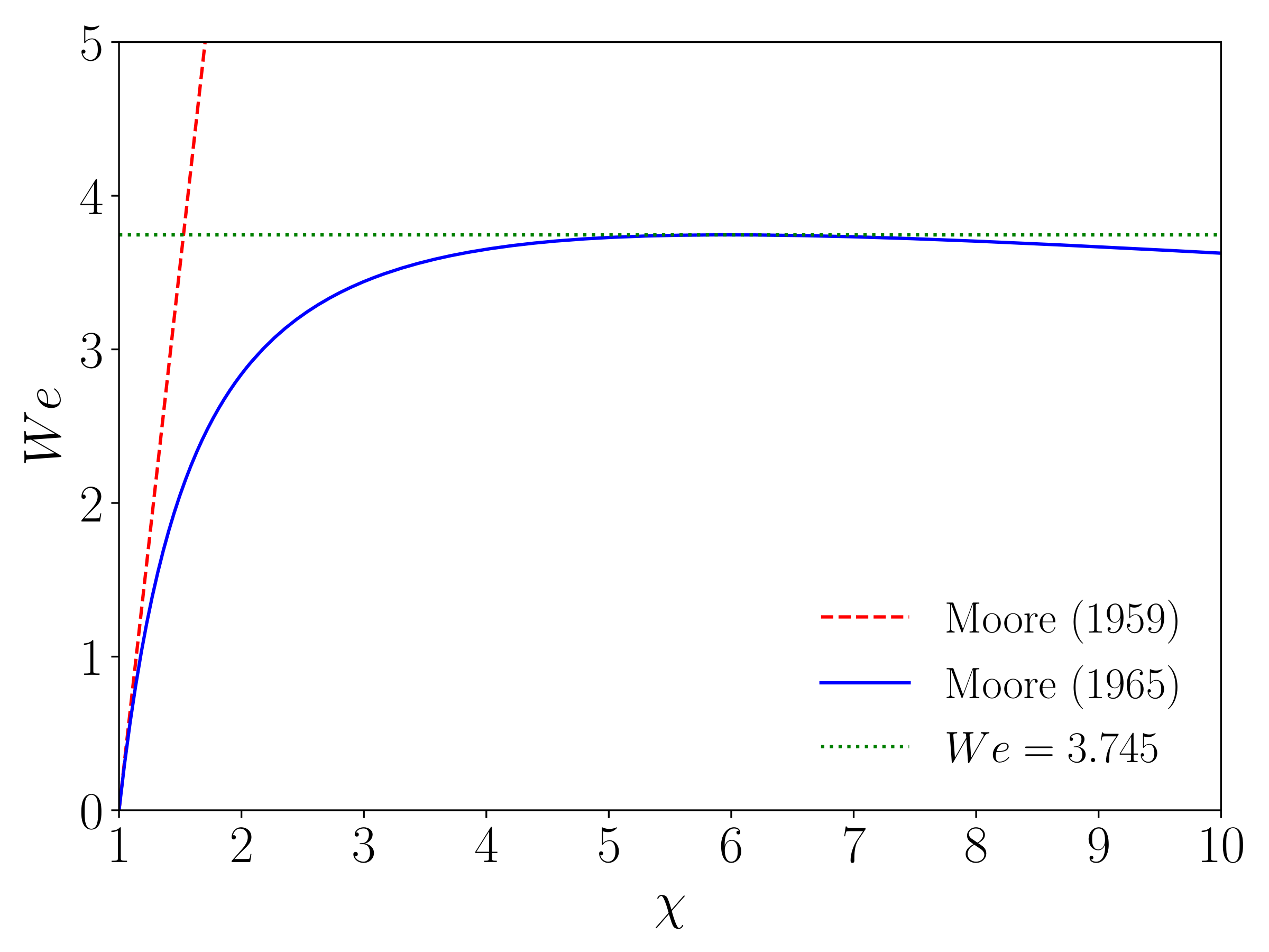
Fig. 6.4 Moore’s bubble shape models

Various bubble shape correlations have been proposed so far. Most of them are extensions of Moore’s model or fitting of the following functional form to experimental data:

(6.59)\[ \chi = 1 + \alpha Eo^{\beta}\]

where \(\alpha\) and \(\beta\) are constants. Some examples are given in Table Constants in aspect ratio correlation.

Table 6.1 Constants in aspect ratio correlation

Source	\(\alpha\)	\(\beta\)	Data
Wellek et al. [WAS66]	0.163	0.757	drops in liquids
Lee and Lee [LL20]	0.21	0.58	deformed bubbles in water flow
Okawa et al. [OTKM03]	1.97	1.3	small bubbles in water
Sugihara et al. [SSSW07]	6.5	1.925	small bubbles in water
Hessenkemper et al. [HZR+21]	0.94	0.0875	deformed bubbles in water flow

Neither \(We\) nor \(Eo\) accounts for the viscous effect on shape deformation. Tadaki and Maeda [TM61] proposed to use a combination of \(Re\) and \(M\) in correlating the bubble aspect ration, i.e.,

(6.60)\[\begin{split} \frac{1}{\chi^{1/3}} = \left\{ \begin{array}{ll} 0.62 & \text{for } 16.5 < T_a \\ 1.36 T_a^{-0.28} & \text{for } 6 < T_a \leq 16.5 \\ 1.14 T_a^{-0.176} & \text{for } 2 < T_a \leq 6 \\ 1 & \text{for } T_a \leq 2 \end{array} \right.\end{split}\]

where \(Ta\) is the Tadaki number defined by

(6.61)\[ Ta = Re M^{0.23}\]

Fan and Tsuchiya [FT90] extended a correlation proposed by Vakrushev and Efremov (1970) as

(6.62)\[\begin{split} \frac{1}{\chi} = \left\{ \begin{array}{ll} 1 & Ta < Ta_1 \\ \{c_1 + c_2 \tanh[c_3 (c_4 - \log_{10} Ta)]\}^m & Ta_1 \leq Ta < Ta_2 \\ 0.24 & Ta_2 \leq Ta \end{array} \right.\end{split}\]

where \(m = 3\), \(Ta_{1} = 1.0, 0.3\), \(Ta_{2} = 40, 20\), \(c_{1} = 0.81\), \(c_{2} = 0.20\), \(c_{3} = 2.0, 1.8\), and \(c_{4} = 0.80, 0.40\), and the former and latter values are for contaminated and clean bubbles, respectively. Aoyama et al. [AHHT16] proposed an alternative way to take into account the viscous effect; they used

(6.63)\[ Ao = Eo^{1.12} Re\]

to correlate \(\chi\) rather than \(Ta\):

(6.64)\[ \chi = \left( 1 + 0.016 Ao \right)^{0.388}\]

Large bubbles cannot maintain an ellipsoidal shape and exhibit the so-called spherical cap shape. The shape and rise velocity of spherical cap bubble will be discussed in Large bubbles in liquid.